Motivation: the other half of uncertainty quantification
The earlier post in this series on uncertainty quantification covered the forward direction: determining the resulting distribution over a simulation’s output, given a known probability distribution over an input. This post treats the mirror-image problem, which is arguably the more common one in practice: given noisy, real-world observations, what can be inferred about an unknown parameter that produced them, and, critically, with what degree of confidence.
That inversion is the mathematical core of an enormous range of applied problems: inferring a patient’s underlying disease risk from noisy clinical measurements, inferring the unknown properties of a material from a small number of experimental tests, or, as this post returns to at the end, inferring the seafloor displacement that triggered a tsunami from a sparse network of ocean pressure sensors, in time to issue a warning before the wave arrives. In each case the same question recurs: given data that constrain the answer only partially and noisily, which values of the unknown parameter are consistent with what was observed, and with what degree of certainty.
Two ways to answer that question
Classical statistics answers this with a point estimate plus a confidence interval. Ordinary least squares, for example, yields a single best-fit coefficient together with a standard error describing how much that estimate would vary were the experiment repeated many times. The claim concerns the long-run behavior of the procedure.
Bayesian inference addresses a different and arguably more directly useful question: the full probability distribution over the unknown parameter, given the data actually observed and not hypothetical repetitions of the experiment. The answer is a distribution, termed the posterior distribution, instead of a single number, and it incorporates uncertainty quantification in the most literal sense.
The structure of Bayes’ theorem
Everything in this post follows from one identity, due originally to (Bayes & Price, 1763). For an unknown parameter $\theta$ and observed data $D$,
\[p(\theta \mid D) = \frac{p(D \mid \theta)\, p(\theta)}{p(D)} \;\propto\; \underbrace{p(D \mid \theta)}_{\text{likelihood}} \cdot \underbrace{p(\theta)}_{\text{prior}}.\]Each term is doing a specific, interpretable job:
- $p(\theta)$, the prior, encodes what was believed about $\theta$ before observing this data: physical bounds, results from previous studies, or, as in the examples below, deliberately weak and close to agnostic beliefs where prior assumptions should not dominate.
- $p(D \mid \theta)$, the likelihood, is the probability of seeing this specific data were $\theta$ the true value. At this point a physical or statistical model of the measurement process enters.
- $p(\theta \mid D)$, the posterior, is the answer: the full distribution of plausible $\theta$ values given what was actually observed, obtained by weighting the prior by how well each candidate $\theta$ explains the data.
- $p(D)$, the evidence, is a normalizing constant (the probability of the data, integrated over all possible $\theta$), and it is precisely the term that makes computing the posterior directly intractable for all but the simplest models, since it requires integrating over every possible parameter value. That intractability is the practical obstacle the remainder of this post addresses.
A bridge from familiar ground: MAP estimation as regularized regression
Before any computational method is introduced, one connection deserves statement. The maximum a posteriori (MAP) estimate, the single most probable value of $\theta$ under the posterior, connects directly to a result from the optimization post in this series. Taking the log of Bayes’ theorem (dropping the constant $p(D)$, which does not affect where the maximum is),
\[\hat{\theta}_{\text{MAP}} = \arg\max_\theta \Big[ \log p(D \mid \theta) + \log p(\theta) \Big].\]If the likelihood is Gaussian and the prior on $\theta$ is also Gaussian with mean zero, this becomes exactly ridge-regularized least squares: the log-likelihood term is (up to constants) the familiar sum of squared residuals, and the log-prior term is exactly an $L_2$ penalty on $\theta$. Concretely, with $D = (X, y)$, $y \mid \theta \sim \mathcal{N}(X\theta, \sigma^2 I)$, and $\theta \sim \mathcal{N}(0, \tau^2 I)$,
\[\hat{\theta}_{\text{MAP}} = \arg\min_\theta \left[ \frac{1}{2\sigma^2}\lVert y - X\theta \rVert_2^2 + \frac{1}{2\tau^2}\lVert \theta \rVert_2^2 \right] = \arg\min_\theta \left[ \lVert y - X\theta \rVert_2^2 + \lambda \lVert \theta \rVert_2^2 \right], \quad \lambda = \frac{\sigma^2}{\tau^2},\]which is precisely ridge regression with regularization strength $\lambda = \sigma^2/\tau^2$. Regularization, viewed through a Bayesian lens, is an informative prior. The equivalence is useful, since it implies that every regularization technique from classical statistics and machine learning admits a direct Bayesian interpretation, and conversely.
Why the posterior usually cannot be computed directly
For anything beyond a small number of textbook “conjugate prior” cases, the posterior distribution has no closed form. The normalizing constant $p(D)$ requires integrating the likelihood multiplied by the prior over every possible parameter value, which is analytically intractable outside a small number of special cases. The standard practical solution is to sample from the posterior instead of computing it in closed form, using Markov Chain Monte Carlo (MCMC).
The Metropolis-Hastings algorithm, from scratch
The idea, due to Metropolis and colleagues in 1953 (Metropolis et al., 1953) and generalized by Hastings in 1970 (Hastings, 1970), is to construct a Markov chain in parameter space that, if run sufficiently long, visits each region of the posterior with a frequency proportional to its posterior probability, without ever computing the intractable normalizing constant.
In its general Metropolis-Hastings form, the algorithm draws a candidate $\theta’$ from a proposal density $q(\theta’ \mid \theta)$ and accepts it with probability $\min(1, r)$, where
\[r = \frac{p(D \mid \theta')\, p(\theta')\, q(\theta \mid \theta')}{p(D \mid \theta)\, p(\theta)\, q(\theta' \mid \theta)}.\]When the proposal is symmetric, $q(\theta’ \mid \theta) = q(\theta \mid \theta’)$, the proposal terms cancel, and the method reduces to the original random-walk Metropolis algorithm, which is the version used throughout this post. At each step, given a current position $\theta$:
- Propose a new candidate $\theta’ = \theta + \epsilon$, where $\epsilon$ is drawn from a simple symmetric distribution (e.g. a Gaussian centered at zero).
- Compute the acceptance ratio $r = \dfrac{p(D \mid \theta’)\, p(\theta’)}{p(D \mid \theta)\, p(\theta)}$. The intractable constant $p(D)$ cancels exactly, since it appears in both numerator and denominator. This cancellation is what makes the algorithm viable: it never requires the overall normalization of the posterior, only the relative posterior density at two points.
- Accept the proposal with probability $\min(1, r)$; otherwise stay at $\theta$.
def metropolis_hastings(log_post_fn, theta0, n_samples, step_sizes, rng):
    theta = np.array(theta0, dtype=float)
    current_lp = log_post_fn(*theta)
    samples = np.zeros((n_samples, len(theta)))
    n_accept = 0
    for i in range(n_samples):
        proposal = theta + rng.normal(0, step_sizes)
        proposal_lp = log_post_fn(*proposal)
        log_accept_ratio = proposal_lp - current_lp   # working in log-space
                                                        # for numerical stability
        if np.log(rng.uniform()) < log_accept_ratio:
            theta = proposal
            current_lp = proposal_lp
            n_accept += 1
        samples[i] = theta
    return samples, n_accept / n_samples
Working entirely in log-space (log-posterior, log-acceptance-ratio) instead of with raw probabilities is standard, and it matters numerically: posterior densities routinely involve products of many small probabilities, which underflow to exactly zero in floating-point arithmetic if computed directly; sums of log-probabilities do not have this problem.
Part A: Inferring a wave source from noisy sensor data
A physically motivated example makes this concrete, and connects directly to the HPC post in this series and its wave-propagation simulation. Consider a simplified inverse problem: a wave pulse of unknown amplitude $A$ originates at an unknown location $x_0$, and a network of sensors at known positions records the peak amplitude and arrival time of the pulse as it passes. The task is to infer $A$ and $x_0$ from the noisy sensor readings alone.
The setup is a deliberately simplified version of the inverse problem underlying real tsunami early-warning systems: infer an unknown source from sparse, noisy sensor observations, fast enough to matter.
The forward model
SENSOR_POSITIONS = np.array([1.0, 2.5, 4.0, 6.0, 8.5])
WAVE_SPEED = 2.0

def forward_model(amplitude, x0):
    dist = np.abs(SENSOR_POSITIONS - x0)
    peak_amp = amplitude / (1.0 + 0.3 * dist)      # geometric spreading/damping
    arrival_time = dist / WAVE_SPEED
    return peak_amp, arrival_time
Synthetic “observed” data is generated from a known true source ($A=3.0$, $x_0=0.2$), corrupted with realistic Gaussian sensor noise. Recovering known parameters from synthetic data is the standard means of validating an inverse-problem pipeline: because the ground truth is known by construction, whether the inference procedure recovers it can be checked directly.
Likelihood and prior
def log_likelihood(amplitude, x0):
    pred_amp, pred_time = forward_model(amplitude, x0)
    ll_amp = -0.5 * np.sum(((obs_amp - pred_amp) / NOISE_STD_AMP) ** 2)
    ll_time = -0.5 * np.sum(((obs_time - pred_time) / NOISE_STD_TIME) ** 2)
    return ll_amp + ll_time

def log_prior(amplitude, x0):
    if not (0.0 < amplitude < 10.0):
        return -np.inf
    if not (-2.0 < x0 < 2.0):
        return -np.inf
    return 0.0   # flat (uniform) prior within physically reasonable bounds
The Gaussian log-likelihood here is not an arbitrary modeling choice. It follows directly from assuming independent, normally distributed measurement noise on each sensor reading, the standard assumption for instrument noise. That assumption is often justified by a central limit argument when the noise is the sum of many small independent error sources.
Because the forward model is nonlinear in $x_0$, this posterior has no closed form, and sampling is the natural way to characterize it.
Running the sampler
N_SAMPLES = 60000
BURN_IN = 10000
samples, accept_rate = metropolis_hastings(
    log_posterior, theta0=[1.0, 0.0], n_samples=N_SAMPLES,
    step_sizes=[0.15, 0.1], rng=rng
)
posterior = samples[BURN_IN:]   # discard burn-in before computing summaries
MCMC acceptance rate: 0.446
Posterior amplitude: mean=2.948, 95% CI=[2.692, 3.213]  (true=3.0)
Posterior x0:        mean=0.224, 95% CI=[0.085, 0.362]  (true=0.2)
Both true parameter values fall comfortably within their respective 95% credible intervals, and the posterior means are close to the ground truth. A correctly implemented inference pipeline should produce exactly this, so the result serves as a validation of the method and not only as a demonstration.
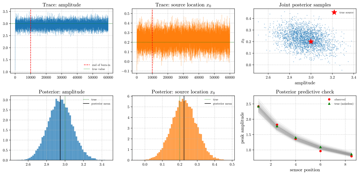
Figure 1: Top row, trace plots for both parameters, showing the position of the chain at every iteration with the true value overlaid, together with the joint posterior sample cloud. Bottom row, marginal posterior histograms and a posterior predictive check: sensor readings forward-simulated from 200 random posterior draws (gray) against the actual noisy observations (red) and the true noiseless signal (green). The gray envelope contains the observations, which is the relevant qualitative check; if it did not, the model itself, and not only the inferred parameters, would be suspect.
Interpreting the diagnostics
Three diagnostics deserve attention, since they form the routine practice of running a sampler correctly:
- Acceptance rate $\approx 0.446$ sits in a reasonable range. If the proposal step size is too large, almost every proposal falls in a low-probability region and is rejected, so the acceptance rate collapses toward zero and the chain barely moves. If it is too small, almost every proposal is accepted, but each step covers so little ground that the chain explores the posterior very slowly. A commonly cited heuristic for random-walk Metropolis targets roughly 20 to 50% acceptance (Roberts et al., 1997), although the appropriate value depends on the dimensionality and shape of the posterior. The figure is a diagnostic to be checked, not a target to be optimized.
- Burn-in (discarding the first 10,000 of 60,000 samples above) exists because the chain starts at an arbitrary initial point and not at a sample from the posterior, so the early samples still reflect that starting point. The trace plots in Figure 1 make this directly visible at the point where the chain stops trending and settles into stable, noisy variation about a fixed level.
- The joint posterior scatter (top-right panel) shows clear correlation structure between $A$ and $x_0$, information that a point estimate alone would discard entirely but that carries physical significance: it identifies which combinations of source parameters are difficult to distinguish given the geometry of this sensor network, which is directly actionable in designing an improved sensor layout.
Part B: Bayesian linear regression on real patient data
To complement the synthetic inverse problem with real data, this section turns to the scikit-learn diabetes dataset: 442 real patients, 10 standardized clinical measurements (age, sex, BMI, blood pressure, six blood serum measurements), and a target variable measuring disease progression one year after baseline.
Classical OLS baseline
ols = LinearRegression(fit_intercept=False).fit(X, y_c)
resid = y_c - X @ ols.coef_
sigma2_hat = np.sum(resid ** 2) / (n - d)
ols_se = np.sqrt(np.diag(sigma2_hat * np.linalg.inv(X.T @ X)))
The Bayesian version
An independent, zero-mean Gaussian prior with variance $\tau^2 = 4$ is placed on each (standardized) regression coefficient, a direct implementation of the equivalence between MAP estimation and ridge regression derived above. The noise standard deviation $\sigma$ is fixed at its plug-in OLS estimate, $\hat{\sigma} = 0.7024$, an empirical-Bayes choice. An earlier version of this post fixed $\sigma = 1.0$; because the target is standardized and the model explains about half of its variance, the residual standard deviation is closer to 0.7, and $\sigma = 1$ widened every credible interval by roughly a factor of 1.4.
With a Gaussian likelihood, a Gaussian prior, and $\sigma$ held fixed, this model is conjugate: the posterior is itself Gaussian, with covariance $\Sigma_{\text{post}} = \left(X^\top X/\sigma^2 + I/\tau^2\right)^{-1}$ and mean $\Sigma_{\text{post}} X^\top y/\sigma^2$. The argument above that the posterior usually has no closed form therefore applies to Part A, not to Part B. MCMC is used here deliberately as a check: because the exact answer is known, the sampler’s output can be compared against it directly.
TAU2 = 4.0                              # prior variance on each coefficient
NOISE_STD = float(np.sqrt(sigma2_hat))  # plug-in OLS estimate of sigma

def log_posterior_reg(beta):
    resid = y_c - X @ beta
    log_lik = -0.5 * np.sum(resid ** 2) / NOISE_STD ** 2
    log_prior_beta = -0.5 * np.sum(beta ** 2) / TAU2
    return log_lik + log_prior_beta

# Closed-form Gaussian posterior: used as an exact check and to shape the proposal
post_cov = np.linalg.inv(X.T @ X / NOISE_STD ** 2 + np.eye(d) / TAU2)
post_mean = post_cov @ (X.T @ y_c) / NOISE_STD ** 2
The sampler is again random-walk Metropolis, now in the full 10-dimensional coefficient space. Several serum measurements (notably s1 and s2, and to a lesser degree s3 through s5) are strongly collinear, so an isotropic random walk mixes very slowly along their joint direction. The proposal is therefore a correlated Gaussian shaped like the posterior covariance and scaled by $2.38^2/d$ with $d = 10$, the standard scaling for random-walk Metropolis (Roberts et al., 1997). The proposal remains symmetric, so the acceptance ratio is unchanged. The chain runs for 40,000 iterations, of which the first 8,000 are discarded as burn-in:
N_SAMPLES_REG = 40000
BURN_IN_REG = 8000
prop_chol = np.linalg.cholesky((2.38 ** 2 / d) * post_cov)
reg_samples, reg_accept = mh_vector(
    log_posterior_reg, np.zeros(d), N_SAMPLES_REG, prop_chol, rng=rng
)
reg_posterior = reg_samples[BURN_IN_REG:]   # 32,000 post-burn-in draws
Noise SD (plug-in OLS estimate): 0.7024
Regression MCMC acceptance rate: 0.261
Effective sample size per coefficient: min 890, max 1104 (of 32000 post-burn-in draws)
Max |MCMC mean - exact mean|: 0.0028; max |MCMC interval end - exact|: 0.0096
Credible / confidence interval width ratio: 1.006 (mean over features)

Feature            OLS coef [95% CI]              Bayes posterior mean [95% credible interval]
age       -0.006 [-0.078, +0.066]      -0.005 [-0.078, +0.067]
sex       -0.148 [-0.222, -0.074]      -0.149 [-0.224, -0.073]
bmi       +0.321 [+0.241, +0.402]      +0.321 [+0.240, +0.404]
bp        +0.200 [+0.121, +0.279]      +0.201 [+0.121, +0.279]
s1        -0.489 [-0.993, +0.015]      -0.472 [-0.968, +0.026]
s2        +0.294 [-0.116, +0.704]      +0.281 [-0.130, +0.696]
s3        +0.062 [-0.195, +0.319]      +0.054 [-0.198, +0.310]
s4        +0.109 [-0.086, +0.305]      +0.110 [-0.090, +0.308]
s5        +0.464 [+0.256, +0.672]      +0.456 [+0.246, +0.670]
s6        +0.042 [-0.038, +0.122]      +0.042 [-0.035, +0.124]
The acceptance rate of 0.261 is close to what the $2.38^2/d$ scaling is designed to produce in ten dimensions. The effective sample size, which accounts for autocorrelation in the chain, ranges from 890 to 1104 per coefficient out of 32,000 post-burn-in draws, which is ample for estimating means and 95% intervals. Most importantly, the MCMC summaries match the exact conjugate posterior: the largest discrepancy in a posterior mean is 0.0028, and the largest discrepancy in an interval endpoint is 0.0096, both small relative to the interval widths. These scripts were run on an AMD Ryzen 7 6800H laptop under WSL2 (Ubuntu 26.04) with Python 3.12.14, NumPy 2.5.3, SciPy 1.18.1, and scikit-learn 1.9.1, using single-threaded BLAS.
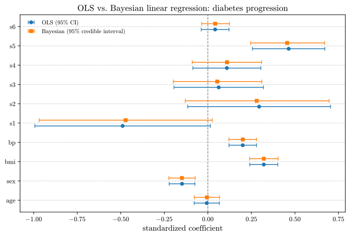
Figure 2: OLS point estimates with 95% confidence intervals (blue) and Bayesian posterior means with 95% credible intervals (orange), for all 10 standardized clinical features. sex, bmi, bp (blood pressure), and s5 have intervals that exclude zero under both approaches, and are the features most clearly associated with disease progression in this cohort.
Why the estimates agree closely here, and when they would not
The OLS and Bayesian estimates land nearly on top of each other in this example: the credible intervals are, on average, 1.006 times as wide as the corresponding confidence intervals. This agreement has a clear explanation. With a weak (large-variance, $\tau^2=4$) Gaussian prior and a reasonably large sample size ($n=442$), the likelihood dominates the posterior, and the posterior is approximately Gaussian, centered near the maximum-likelihood estimate with covariance close to its sampling covariance. This is the content of the Bernstein-von Mises theorem, a general asymptotic result that is not specific to this dataset (Efron & Hastie, 2016). The small shifts that remain, visible mainly in the collinear coefficients s1, s2, and s5, reflect the mild shrinkage that the prior applies where the data constrain individual coefficients least.
The Bayesian approach is advantageous in the regimes where this does not hold: small sample sizes (where the prior meaningfully constrains an otherwise poorly determined estimate), informative priors built from real external knowledge (a previous clinical study’s results feeding directly into this one), and whenever a full posterior over a downstream, nonlinear quantity is required. A Bayesian analysis yields the exact distribution of any function of the samples at negligible additional cost, by applying the function to every posterior draw, whereas a classical approach would require a separate and often approximate argument, such as the delta method, to propagate uncertainty through a nonlinear transformation. A classical, non-Bayesian alternative that provides a useful point of contrast is the bootstrap, which constructs confidence intervals by resampling the data without specifying a prior (Efron, 1979).
Connecting back: a recent breakthrough in real-time Bayesian inversion
The HPC post earlier in this series described the 2025 Gordon Bell Prize-winning tsunami early-warning system built at LLNL, running on the El Capitan exascale supercomputer (Lawrence Livermore National Laboratory, 2025). The toy wave-source inference problem in Part A above is a deliberately simplified analogue of the task that system addresses: given real-time seafloor pressure sensor readings, infer the unknown source that best explains them, with quantified uncertainty, and use that inferred source to forecast the resulting wave. The operational framework is a Bayesian inversion built on a physics-based forward model, the same structure developed in this post, but at a vastly larger scale and under severe time constraints (Lawrence Livermore National Laboratory, 2025)(Newswise, 2025).
The simplified example also avoids the central computational difficulty. Random-walk Metropolis, as implemented above, would be far too slow for a real-time, life-safety application. Sixty thousand samples of a two-parameter posterior require a fraction of a second on a laptop, whereas a full-physics tsunami inversion cannot be run tens of thousands of times sequentially within the short time available before a wave arrives. As described in the published accounts, the LLNL framework addresses this by moving the expensive physics-based computation into an offline precomputation stage on El Capitan, so that the online inference step, performed once sensor data arrive, is very fast (Lawrence Livermore National Laboratory, 2025)(Newswise, 2025). The underlying Bayesian formulation of the inverse problem is the one presented here and treated in general form in (Tarantola, 2005); the engineering contribution lies in reorganizing the computation so that inference is fast enough to support a warning.
Summary Notes and Highlights
- Bayesian inference reframes the question, replacing a single answer with the full distribution of plausible answers given what was actually observed. That question differs from, and is often more useful than, a classical point estimate accompanied by a confidence interval.
- MAP estimation is regularized regression in another form: an explicit prior is mathematically equivalent to an explicit regularization penalty, which provides a useful bridge for readers approaching the subject from optimization.
- Metropolis-Hastings sidesteps the intractable normalizing constant by working entirely with ratios of posterior densities, which is the key mathematical step that makes MCMC computationally feasible.
- Acceptance rate, trace plots, burn-in, and effective sample size are diagnostics to be checked, not boilerplate. A poorly tuned sampler can silently produce a plausible-looking but incorrect posterior, and these are the tools for detecting that outcome. When a closed-form posterior exists, as in Part B, comparing against it is the most direct check of all.
- Posterior predictive checks, which simulate data from posterior draws and compare it against what was actually observed, are among the most underused and most valuable checks in applied Bayesian work.
- Bayesian and classical estimates converge given sufficient data and a weak prior, as the Bernstein-von Mises theorem predicts and the diabetes example confirms. The advantage of the Bayesian approach appears in small samples, with informative priors, and when propagating uncertainty through nonlinear downstream quantities.
References
The foundational identity underlying this entire post is due to (Bayes & Price, 1763). The Metropolis-Hastings algorithm follows (Metropolis et al., 1953) and its generalization by (Hastings, 1970), with practical acceptance-rate targets justified theoretically in (Roberts et al., 1997). (Gelman et al., 2013) is the standard modern reference for Bayesian modeling, MCMC diagnostics, and posterior predictive checks, and (Tarantola, 2005) is the classical reference connecting Bayesian inference to physical inverse problems specifically. (Efron & Hastie, 2016) gives an especially clear, modern treatment of the Bayesian/frequentist correspondence discussed above, and (Efron, 1979) introduces the bootstrap as a classical non-Bayesian point of contrast. The Gordon Bell Prize-winning tsunami-forecasting system referenced throughout is documented in (Lawrence Livermore National Laboratory, 2025) and (Newswise, 2025).
- Bayes, T., & Price, R. (1763). An Essay Towards Solving a Problem in the Doctrine of Chances. Philosophical Transactions of the Royal Society of London, 53, 370–418.
- Metropolis, N., Rosenbluth, A. W., Rosenbluth, M. N., Teller, A. H., & Teller, E. (1953). Equation of State Calculations by Fast Computing Machines. Journal of Chemical Physics, 21(6), 1087–1092.
- Hastings, W. K. (1970). Monte Carlo Sampling Methods Using Markov Chains and Their Applications. Biometrika, 57(1), 97–109.
- Roberts, G. O., Gelman, A., & Gilks, W. R. (1997). Weak Convergence and Optimal Scaling of Random Walk Metropolis Algorithms. Annals of Applied Probability, 7(1), 110–120.
- Efron, B., & Hastie, T. (2016). Computer Age Statistical Inference. Cambridge University Press.
- Efron, B. (1979). Bootstrap Methods: Another Look at the Jackknife. Annals of Statistics, 7(1), 1–26.
- Lawrence Livermore National Laboratory. (2025). LLNL, UT & UCSD Win Gordon Bell Prize with Exascale Tsunami Forecasting. https://www.llnl.gov/article/53636
- Newswise. (2025). LLNL, UT & UCSD Win Gordon Bell Prize with Exascale Tsunami Forecasting. https://www.newswise.com/articles/llnl-ut-ucsd-win-gordon-bell-prize-with-exascale-tsunami-forecasting
- Tarantola, A. (2005). Inverse Problem Theory and Methods for Model Parameter Estimation. SIAM.
- Gelman, A., Carlin, J. B., Stern, H. S., Dunson, D. B., Vehtari, A., & Rubin, D. B. (2013). Bayesian Data Analysis (3rd ed.). CRC Press.
Full, executed code for both the wave-source inversion and the diabetes regression comparison is available in bayesian_inference_p8.py.