Motivation
Earlier posts in this series addressed making a single simulation run fast: accelerating the linear algebra (Sherman-Morrison) and choosing a solver that is not constrained by numerical stiffness (stiff ODEs). In practice, however, a single run rarely answers the question at hand. Real inputs, including material properties, boundary conditions, and flight parameters, are uncertain, and propagating that uncertainty through a simulation to determine its effect on the output (the quantity of interest, or QoI) typically requires running the simulation many times.
If a single high-fidelity run takes hours on a cluster, evaluating it tens of thousands of times for a Monte Carlo uncertainty study is infeasible. Uncertainty quantification (UQ) provides methods for closing this gap, and one of its central tools is surrogate modeling: replacing the expensive simulation with an inexpensive and accurate substitute constructed from a modest number of well-chosen runs. This post introduces one of the standard techniques for building such surrogates, polynomial chaos expansion (PCE) (Wiener, 1938)(Ghanem & Spanos, 1991), from first principles using a worked example.
The setup
Suppose an uncertain input parameter $x$, for example a normalized material property or geometric tolerance, is distributed as $x \sim \mathrm{Uniform}(-1, 1)$, and the simulation output, the quantity of interest, is some function $f(x)$. In real applications, $f$ is an expensive black box, such as a CFD solve or a finite-element structural analysis. Here, to keep the mathematics inspectable, a smooth substitute with a sharp response feature is used, so that the convergence behavior reported below is not trivially favorable. The test function is Runge’s function:
\[f(x) = \frac{1}{1 + 25x^2}.\]The goal of UQ is typically to estimate statistics of the output induced by the uncertainty in the input, most commonly the mean and variance,
\[\mathbb{E}[f(x)], \qquad \mathrm{Var}[f(x)].\]For this function, both have closed forms under the uniform density on $[-1,1]$, which provide exact references for the error measurements below:
\[\mathbb{E}[f] = \frac{\arctan 5}{5} \approx 0.274680, \qquad \mathrm{Var}[f] = \frac{1}{2}\left(\frac{1}{26} + \frac{\arctan 5}{5}\right) - \mathbb{E}[f]^2 \approx 0.081122.\]The direct approach is Monte Carlo: draw many samples of $x$, evaluate $f$ at each, and compute sample statistics. It is simple and general, but its error decays only as $O(N^{-1/2})$ in the number of simulation calls $N$, which is prohibitively slow when each call is expensive.
Polynomial chaos expansion
The principle behind PCE is to expand the output as a series in polynomials that are orthogonal with respect to the probability distribution of the input,
\[f(x) \approx \sum_{j=0}^{p} c_j\, \Phi_j(x).\]For $x \sim \mathrm{Uniform}(-1,1)$, the appropriate orthogonal family is the Legendre polynomials $\Phi_j = P_j$, which satisfy
\[\int_{-1}^{1} P_i(x) P_j(x)\, dx = \|P_j\|^2\, \delta_{ij}, \qquad \|P_j\|^2 = \frac{2}{2j+1}.\]Different input distributions call for different polynomial families, a correspondence known as the Askey scheme (Xiu & Karniadakis, 2002): Hermite polynomials for Gaussian inputs, Laguerre polynomials for exponential inputs, and so on. An ill-matched polynomial family for a given distribution still converges in principle, but forfeits the fast convergence that makes PCE worthwhile.
Because the basis is orthogonal, the expansion coefficients are projections,
\[c_j = \frac{1}{\|P_j\|^2}\int_{-1}^{1} f(x)\, P_j(x)\, dx .\]The uniform density $1/2$ cancels between numerator and denominator here, since both the projection and the norm could equally be taken with respect to $dx/2$; the code below uses the unweighted form, dividing the quadrature sum by $|P_j|^2 = 2/(2j+1)$. In practice, the integral is evaluated numerically by Gauss-Legendre quadrature. An $m$-node Gauss-Legendre rule integrates polynomials of degree up to $2m-1$ exactly, but the integrand $f\,P_j$ is not a polynomial when $f$ is Runge’s function, so each computed coefficient carries a quadrature error and the projection is approximate. The implementation below uses $m = p + 5$ nodes for an order-$p$ expansion, so the number of model evaluations grows linearly with the polynomial order.
Once the coefficients $c_j$ are known, the mean and variance of the output follow algebraically, with no further sampling. Under the uniform density, $\mathbb{E}[P_j^2] = |P_j|^2/2$, so
\[\mathbb{E}[f] = c_0, \qquad \mathrm{Var}[f] = \sum_{j=1}^{p} c_j^2 \, \frac{\|P_j\|^2}{2} = \sum_{j=1}^{p} \frac{c_j^2}{2j+1}.\]This is the key structural advantage over Monte Carlo: the statistics are a direct algebraic readout of the expansion coefficients, not a separate sampling process layered on top of the surrogate.
Implementation
import numpy as np
from numpy.polynomial import legendre as L

def legendre_basis_eval(order, x):
    """Phi[i, j] = P_j(x_i) for orders 0..order."""
    n_terms = order + 1
    Phi = np.zeros((len(x), n_terms))
    for j in range(n_terms):
        c = np.zeros(n_terms)
        c[j] = 1.0
        Phi[:, j] = L.legval(x, c)
    return Phi

def pce_coefficients(order, f):
    n_quad = order + 5
    nodes, weights = np.polynomial.legendre.leggauss(n_quad)
    fvals = f(nodes)
    Phi = legendre_basis_eval(order, nodes)
    coeffs = np.zeros(order + 1)
    for j in range(order + 1):
        norm_j = 2.0 / (2 * j + 1)  # <P_j, P_j> normalization on [-1, 1]
        coeffs[j] = np.sum(weights * fvals * Phi[:, j]) / norm_j
    return coeffs

def pce_eval(coeffs, x):
    return L.legval(x, coeffs)
Surrogate accuracy
Fitting PCE surrogates of increasing polynomial order against the true response function gives the following:
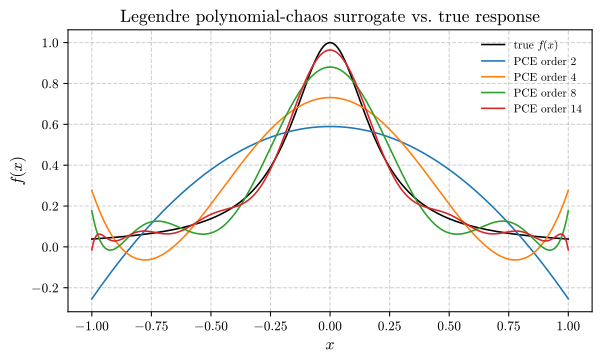
Figure 1: True response $f(x)$ against PCE surrogates of order 2, 4, 8, and 14. Low-order expansions miss the sharp peak near $x=0$; by order 14, the surrogate is visually indistinguishable from the truth.
The low-order surrogates perform worst precisely where $f$ is sharpest. This behavior reflects a deliberate choice of test function: a smoother QoI would likely converge faster still, and a more demanding one was selected so that the convergence results below are not artificially favorable.
PCE vs. Monte Carlo: convergence comparison
The decisive test is efficiency: for a fixed budget of simulation calls, the relevant question is how accurately each method estimates the mean and variance. The errors below are measured against the closed-form references given earlier.
# Exact reference values for f(x) = 1/(1 + 25 x^2), x ~ Uniform(-1, 1)
mean_ref = np.arctan(5.0) / 5.0
var_ref = 0.5 * (1.0 / 26.0 + np.arctan(5.0) / 5.0) - mean_ref**2
# mean_ref = 0.274680, var_ref = 0.081122

for order in range(1, 61):
    c = pce_coefficients(order, f)          # uses order + 5 evaluations
    mean_est = c[0]
    var_est = np.sum((c[1:]**2) * (2.0 / (2 * np.arange(1, len(c)) + 1)) / 2.0)
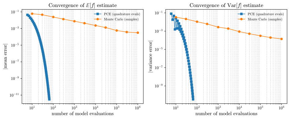
Figure 2: Absolute error in the estimated mean (left) and variance (right) of $f(x)$ as a function of the number of model evaluations, comparing PCE (quadrature-based, orders 1 to 60) against standard Monte Carlo (up to $10^6$ samples, error averaged over 30 repeats). Both axes are log-scaled.
The measured errors in the mean are as follows:
| PCE order $p$ | Evaluations ($p+5$) | Mean error |
|---|---|---|
| 5 | 10 | $9.49 \times 10^{-3}$ |
| 10 | 15 | $1.33 \times 10^{-3}$ |
| 15 | 20 | $1.82 \times 10^{-4}$ |
| 20 | 25 | $2.49 \times 10^{-5}$ |
| 30 | 35 | $4.69 \times 10^{-7}$ |
| 40 | 45 | $8.82 \times 10^{-9}$ |
| 50 | 55 | $1.66 \times 10^{-10}$ |
| 60 | 65 | $3.12 \times 10^{-12}$ |
The variance error behaves similarly: $8.55 \times 10^{-4}$ at order 15 (20 evaluations), $2.34 \times 10^{-6}$ at order 30 (35 evaluations), and $3.39 \times 10^{-11}$ at order 60 (65 evaluations). Monte Carlo, by comparison, gives a mean error of $7.05 \times 10^{-3}$ with $1{,}000$ samples, $1.50 \times 10^{-3}$ with $30{,}000$, and $2.57 \times 10^{-4}$ with $1{,}000{,}000$, following its characteristic $O(N^{-1/2})$ decay.
The PCE error decays geometrically: it falls by a factor of roughly $7$ for every $5$ additional evaluations. At $20$ evaluations, PCE already matches the accuracy that Monte Carlo reaches with a million samples, and about $65$ evaluations bring the error to about $10^{-12}$. This convergence is geometric but not especially fast, and the reason lies in the test function. Runge’s function is analytic on $[-1,1]$, but it has poles at $x = \pm i/5$ in the complex plane, very close to the real interval. The rate of geometric convergence of a Legendre expansion is governed by the distance of the nearest singularity from the interval, so poles this close limit the rate. A QoI whose nearest singularity lies farther away would converge faster; Monte Carlo, in contrast, retains the same $1/\sqrt{N}$ rate regardless of the smoothness of the underlying function.
Limitations
The efficiency of PCE is not unconditional, and the principal failure modes merit explicit statement:
- Curse of dimensionality. With $d$ uncertain inputs, a full tensor-product basis of order $p$ in each variable contains $(p+1)^d = O(p^d)$ terms, while a total-degree basis (all multivariate polynomials of total degree at most $p$) contains $\binom{p+d}{d}$ terms. The total-degree basis is much smaller but still grows rapidly with $d$, so for problems with many uncertain parameters PCE can become less favorable than Monte Carlo. Sparse-grid and adaptive basis-selection methods exist specifically to reduce this growth, at the cost of additional implementation complexity.
- Non-smooth QoIs. If the response has a discontinuity, such as a bifurcation, a phase change, or a contact event, global polynomial expansions converge slowly or exhibit Gibbs-type oscillation; the appropriate remedy is often a localized or piecewise surrogate.
- Correlated or non-standard input distributions require either a different orthogonal polynomial family, in accordance with the Askey scheme, or a prior transform to a standard distribution. An ill-matched basis degrades the convergence rate without producing an outright incorrect answer, which makes the error easy to overlook.
Beyond mean and variance: sensitivity analysis
A further advantage of constructing a PCE surrogate is that, once it exists, higher-order UQ analyses require additional computation on the surrogate, not new simulation runs. Sobol sensitivity indices (Sobol,’ 2001), which measure how much of the output variance is attributable to each individual input and to interactions among inputs, can be read directly from the PCE coefficients in the multi-input case, with no additional model evaluations required (Sudret, 2008). For a single-input problem such as the one above, the distinction is not visible, since the single input trivially explains $100\%$ of the variance. In a realistic multi-parameter engineering study, however, this is often a more actionable output than the mean and variance alone: identifying which one or two input parameters dominate the output uncertainty indicates where further experimentation or tighter manufacturing tolerances should be directed.
Two routes to constructing a PCE surrogate
The projection approach shown above, which uses Gauss quadrature to compute each coefficient by numerical integration, is the classical route when the evaluation points may be chosen freely; its accuracy is limited only by truncation and quadrature error. In some engineering settings, however, a fixed set of simulation runs is given, such as a legacy design-of-experiments campaign, and new evaluation points cannot be selected. In that case, PCE coefficients are instead estimated by least-squares regression: fitting the coefficients $c_j$ that best match the existing $(x_i, f(x_i))$ data in a least-squares sense, using the same Legendre basis functions. Regression-based PCE recovers similar convergence benefits when the sample points are well distributed and outnumber the basis terms by a sufficient margin, and its accuracy degrades gradually when the data are sparse or unevenly distributed. This makes it a useful, practical alternative when quadrature is unavailable (Xiu, 2010).
Applied implementation notes
Several considerations apply before adopting a PCE library on a real project (chaospy and UQpy are common choices in Python):
- Validate against a held-out sample. Fit the surrogate on one set of points, then assess its predictions on points excluded from fitting. This is the same discipline applied to any regression or machine-learning model, and for the same reason: a surrogate that reproduces only its training quadrature points is of no practical use.
- Consider the trade-off between polynomial order and evaluation budget. Higher order yields faster convergence per basis function, but the number of basis functions itself grows combinatorially with the number of uncertain inputs, so in high-dimensional cases the order must be chosen more conservatively than the single-input example here would suggest.
- Non-uniform, correlated, or bounded-but-non-uniform inputs are common in practice and require either selecting the matching Askey-scheme polynomial family or applying an isoprobabilistic transform, such as the Rosenblatt transform, to map the actual input distribution onto a standard one before building the expansion.
Summary Notes and Highlights
- Surrogate modeling makes uncertainty propagation tractable when the underlying simulation is too expensive to evaluate thousands of times.
- Polynomial chaos expansion constructs that surrogate by projecting the QoI onto polynomials orthogonal with respect to the probability distribution of the input. For smooth QoIs, this yields geometric convergence in place of the fixed $1/\sqrt{N}$ rate of Monte Carlo; for Runge’s function, 20 evaluations matched the accuracy of a million Monte Carlo samples.
- The rate of that convergence depends on the smoothness of the QoI, including the location of its complex singularities, and the overall advantage depends on dimensionality. Both assumptions require checking before PCE is preferred over more robust, if slower, sampling-based alternatives.
Taken together, the three posts so far cover fast linear algebra, stability-aware time integration, and efficient uncertainty propagation: make each simulation call inexpensive, ensure the solver does not silently demand more calls than necessary, and exercise judgment about how many calls a question requires. The next post compares physics-informed neural networks with the classical methods discussed so far.
References
The polynomial-chaos construction used throughout this post traces back to (Wiener, 1938) for Gaussian-type inputs via Hermite polynomials, with (Ghanem & Spanos, 1991) giving the first systematic engineering application. (Xiu & Karniadakis, 2002) establishes the generalized Askey-scheme correspondence between input distributions and orthogonal polynomial families used above, and (Xiu, 2010) gives a thorough textbook treatment of both quadrature- and regression-based coefficient estimation. The sensitivity-analysis discussion draws on (Sobol,’ 2001) for the classic Sobol indices and on (Sudret, 2008), which shows how those indices can be read directly from PCE coefficients without additional simulation runs.
- Wiener, N. (1938). The Homogeneous Chaos. American Journal of Mathematics, 60(4), 897–936.
- Ghanem, R. G., & Spanos, P. D. (1991). Stochastic Finite Elements: A Spectral Approach. Springer.
- Xiu, D., & Karniadakis, G. E. (2002). The Wiener-Askey Polynomial Chaos for Stochastic Differential Equations. SIAM Journal on Scientific Computing, 24(2), 619–644.
- Sobol’, I. M. (2001). Global Sensitivity Indices for Nonlinear Mathematical Models and Their Monte Carlo Estimates. Mathematics and Computers in Simulation, 55(1-3), 271–280.
- Sudret, B. (2008). Global Sensitivity Analysis Using Polynomial Chaos Expansions. Reliability Engineering & System Safety, 93(7), 964–979.
- Xiu, D. (2010). Numerical Methods for Stochastic Computations: A Spectral Method Approach. Princeton University Press.
Full code for this post is available in pce_demo_p3.py.