Motivation
Sustainable Aviation Fuel (SAF) blending studies, fuel-burn optimization, and mission-performance models share a common computational bottleneck: each requires integrating a system of ordinary differential equations (ODEs) that describes the aircraft’s state (mass, velocity, altitude, and various internal dynamic modes) over the course of a flight. Because aircraft mass decreases continuously as fuel burns, the matrix governing these dynamics is not fixed; it drifts over time.
For stiff or tightly coupled formulations, implicit time-stepping schemes are the standard choice, since explicit schemes would demand impractically small time steps for stability (a topic treated in more depth in the next post in this series). Implicit schemes, however, require solving a linear system at every time step. Implemented directly, this means refactoring an $n \times n$ matrix from scratch at each step: an $O(n^3)$ operation repeated hundreds or thousands of times over a full flight-mission simulation.
This post examines a case in which that cost is avoidable. When the time-varying part of the system matrix is low rank, as occurs when a single scalar quantity such as remaining fuel mass enters the dynamics as a coupling, the Sherman-Morrison formula allows the system matrix to be factorized once and the factorization to be reused for the entire simulation, reducing the per-step cost from $O(n^3)$ to $O(n^2)$.
The material is a generalized reconstruction of a numerical approach I used during a graduate research internship at Lawrence Livermore National Laboratory, where the technique accelerated an ODE solver for a sustainable aviation modeling application. The system, data, and code below form a self-contained synthetic reconstruction prepared for this post; none of the material reproduces proprietary code or data.
Setting up the problem
Consider a linear time-varying ODE system:
\[\frac{dy}{dt} = A(t)\, y + b, \qquad A(t) = A_0 + c(t)\, u v^\top .\]Here $y(t) \in \mathbb{R}^n$ is the state vector (velocity perturbations, structural modes, and thermal states, depending on the quantities the model tracks), $A_0$ is a fixed baseline dynamics matrix, and $c(t)\,uv^\top$ is a rank-one correction whose direction ($u, v \in \mathbb{R}^n$) remains fixed while its strength $c(t)$ evolves smoothly over the flight. Physically, $c(t)$ acts as a fuel-mass-dependent coupling coefficient: as fuel is consumed, the aircraft’s mass distribution shifts, and that shift enters the dynamics matrix along a fixed structural direction, scaled by a coefficient that decays over the flight horizon.
Discretizing with backward (implicit) Euler at step size $h$,
\[y_{k+1} = y_k + h\left(A(t_{k+1})\, y_{k+1} + b\right) \quad\Longrightarrow\quad \big(I - hA_{k+1}\big)\, y_{k+1} = y_k + hb,\]and substituting $A_{k+1} = A_0 + c_{k+1}\, uv^\top$, with $c_{k+1} = c(t_{k+1})$, $t_{k+1} = (k+1)h$, and the fixed matrix $B_0 := I - hA_0$, gives
\[M_{k+1}y_{k+1} = y_k + hb, \qquad M_{k+1} = B_0 - hc_{k+1}uv^\top.\]The key structural observation is that $M_{k+1}$ is always a rank-one perturbation of the same fixed matrix $B_0$: the perturbation strength changes at every step, whereas $B_0$ does not.
The Sherman-Morrison formula
For an invertible matrix $B \in \mathbb{R}^{n\times n}$ and vectors $u, v \in \mathbb{R}^n$ such that $B + \alpha uv^\top$ remains invertible, the Sherman-Morrison formula gives the inverse of the rank-one update directly, without a fresh factorization:
\[\left(B + \alpha\, uv^\top\right)^{-1} = B^{-1} - \frac{\alpha\, B^{-1}u\, v^\top B^{-1}}{1 + \alpha\, v^\top B^{-1}u}.\]Derivation sketch. Write $B^{-1}u = p$ and $v^\top B^{-1} = q^\top$, and let $\sigma = 1 + \alpha v^\top B^{-1}u = 1 + \alpha q^\top u$. Multiplying the right-hand side above by $\left(B + \alpha uv^\top\right)$ and expanding term by term,
\[\left(B^{-1} - \frac{\alpha\, p q^\top}{\sigma}\right)\left(B + \alpha uv^\top\right) = I + \alpha B^{-1} u v^\top - \frac{\alpha}{\sigma}\, p q^\top B - \frac{\alpha^2}{\sigma}\, p q^\top u v^\top .\]Using $q^\top B = v^\top$ and $q^\top u = v^\top B^{-1}u = (\sigma - 1)/\alpha$, the last two terms combine to $-\dfrac{\alpha}{\sigma}pv^\top!\left(1 + \alpha \dfrac{\sigma-1}{\alpha}\right) = -\alpha pv^\top$, which exactly cancels the second term $\alpha B^{-1}uv^\top = \alpha pv^\top$. What remains is the identity matrix, confirming the formula.
Why this is computationally important. The inverse never needs to be formed explicitly. Applied to a right-hand side $r$, the formula reads
\[\left(B_0 + \alpha\, uv^\top\right)^{-1} r = z - \frac{\alpha\,(v^\top z)}{1 + \alpha\, v^\top p}\, p, \qquad z = B_0^{-1} r, \quad p = B_0^{-1} u .\]Once $B_0$ has been LU-factorized, at a cost of one $O(n^3)$ factorization, the vector $p$ and the scalar $v^\top p$ can be computed once and stored, because neither depends on the step. Each new value $\alpha = -hc_{k+1}$ then costs only
- one pair of triangular solves with the stored LU factors to obtain $z$: $O(n^2)$;
- two dot products and one vector update: $O(n)$.
No refactorization is required. The $O(n^3)$ cost is paid exactly once, at the start of the simulation, instead of at every one of the $T$ time steps. For a simulation with $T$ steps, this reduces an $O(Tn^3)$ algorithm to an $O(n^3 + Tn^2)$ one.
Implementation
Both solvers evaluate the coupling coefficient at $t_{k+1} = (k+1)h$, as backward Euler requires.
import numpy as np
from scipy.linalg import lu_factor, lu_solve

def solve_naive(A0, u, v, b, y0, h, steps, T):
    """Refactor the full system matrix from scratch at every step: O(n^3) per step."""
    n = len(y0)
    y = y0.copy()
    traj = [y.copy()]
    for k in range(steps):
        t = (k + 1) * h          # backward Euler evaluates A at t_{k+1}
        c = fuel_burn_coeff(t, T)
        Ak = A0 + c * np.outer(u, v)
        M = np.eye(n) - h * Ak
        rhs = y + h * b
        y = np.linalg.solve(M, rhs)
        traj.append(y.copy())
    return np.array(traj)

def solve_sherman_morrison(A0, u, v, b, y0, h, steps, T):
    """Factor B0 = I - h A0 once, then apply the rank-one Sherman-Morrison
    correction at each step: O(n^3) once, then O(n^2) per step."""
    B0 = np.eye(len(y0)) - h * A0
    lu_piv = lu_factor(B0)            # the single O(n^3) factorization
    p = lu_solve(lu_piv, u)           # B0^{-1} u, reused every step
    vp = v @ p
    y = y0.copy()
    traj = [y.copy()]
    for k in range(steps):
        t = (k + 1) * h
        alpha = -h * fuel_burn_coeff(t, T)
        z = lu_solve(lu_piv, y + h * b)       # O(n^2)
        y = z - (alpha * (v @ z) / (1.0 + alpha * vp)) * p
        traj.append(y.copy())
    return np.array(traj)
The fuel_burn_coeff function models the decaying coupling strength as fuel is consumed over the flight horizon $T$:
def fuel_burn_coeff(t, T, c0=2.0):
    return c0 * (1.0 - t / T)
Correctness check
Before the speedup can be relied upon, both methods must be confirmed to produce the same trajectory up to floating-point round-off. Running both solvers on an identical $30$-dimensional system over $400$ steps gives a maximum absolute deviation between the two trajectories of $1.948 \times 10^{-11}$, a magnitude consistent with floating-point round-off and not with a real discrepancy between the methods. This agreement is expected, since Sherman-Morrison is an exact algebraic identity, not an approximation.
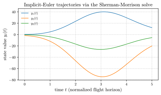
Figure 1: Trajectories of the first three state components under the Sherman-Morrison-accelerated implicit Euler scheme.
Benchmark: measured performance
Wall-clock time for both approaches was measured across system sizes $n \in {20, 40, 80, 160, 320, 640}$, running $150$ implicit Euler steps for each and reporting the median of $5$ repeats. The runs used an AMD Ryzen 7 6800H under WSL2 (Ubuntu 26.04) with Python 3.12.14, NumPy 2.5.3, and SciPy 1.18.1, with BLAS restricted to a single thread (OMP_NUM_THREADS, OPENBLAS_NUM_THREADS, and MKL_NUM_THREADS set to 1):
n=  20  naive=0.0115s  sherman-morrison=0.0143s  speedup=0.81x
n=  40  naive=0.0192s  sherman-morrison=0.0071s  speedup=2.69x
n=  80  naive=0.0354s  sherman-morrison=0.0092s  speedup=3.86x
n= 160  naive=0.1245s  sherman-morrison=0.0170s  speedup=7.33x
n= 320  naive=0.6225s  sherman-morrison=0.0205s  speedup=30.33x
n= 640  naive=4.6166s  sherman-morrison=0.0541s  speedup=85.31x
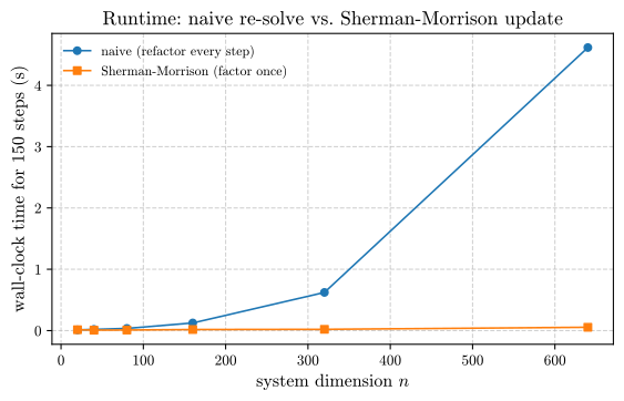
Figure 2: Wall-clock time for 150 implicit Euler steps, naive re-solve vs. Sherman-Morrison rank-one update, across system dimension $n$.
The speedup grows monotonically with $n$, from $2.69\times$ at $n = 40$ to $85.31\times$ at $n = 640$, consistent with the $O(n^3)$ against $O(n^2)$ per-step scaling: each doubling of $n$ multiplies the naive cost by a factor approaching $8$ at the largest sizes, while the Sherman-Morrison cost grows far more slowly. The smallest case is the exception. At $n = 20$, the Sherman-Morrison solver is slower ($0.81\times$), because for so small a system the arithmetic is negligible and the run time is dominated by fixed per-call overhead: the SciPy lu_solve wrapper, Python-level bookkeeping, and array allocation cost more than the dense solve they replace. The asymptotic advantage becomes visible only once the $O(n^3)$ work is large enough to outweigh these constants. The exact multipliers also depend on the BLAS backend, cache behavior, and the number of steps, so they should be read as specific to this machine and configuration.
Conditions for applicability
The Sherman-Morrison structure is common in practice, but it is not universal. It applies cleanly when:
- The time-varying part of the system matrix is low rank (rank one, or rank $k$ via the generalized Woodbury identity below), and
- The direction of the perturbation is fixed, with only its magnitude changing over time, as with a single scalar physical quantity such as fuel mass, a temperature-dependent stiffness, or a single damaged structural element.
The formula offers no advantage if the entire matrix changes at every step with no shared low-rank structure. In that regime, the available options are per-step refactorization or the exploitation of a different structure entirely, such as sparsity, banded matrices, or iterative Krylov methods.
Asymptotic complexity
The argument for this technique rests on the asymptotic comparison, which is set out explicitly below: at each step, the naive approach requires a fresh $O(n^3)$ factorization, while the Sherman-Morrison approach uses one initial $O(n^3)$ factorization and then $O(n^2)$ work per step.
| Operation | Naive re-solve | Sherman-Morrison |
|---|---|---|
| One-time setup | - | $O(n^3)$ (factor $B_0$) |
| Cost per time step | $O(n^3)$ (refactor $M_k$) | $O(n^2)$ (two triangular solves) |
| Total over $T$ steps | $O(Tn^3)$ | $O(n^3 + Tn^2)$ |
| Break-even point | - | asymptotically favorable for any $T \ge 2$; in practice set by constants and per-call overhead |
In leading-order terms, the Sherman-Morrison approach pays for one factorization plus $T$ cheap solves, whereas the naive approach pays for $T$ factorizations, so the advantage holds asymptotically for any simulation with two or more steps and grows with $T$. The practical break-even point is instead determined by constant factors and overhead, which the asymptotic count ignores. The $n = 20$ benchmark above illustrates this: with only $20$ unknowns, the fixed cost of each library call outweighs the savings in arithmetic, and the naive solver is faster. For the long time horizons and moderate-to-large state dimensions typical of flight-mission simulations, the Sherman-Morrison approach is decisively faster.
A note on numerical stability
The Sherman-Morrison formula has a denominator, $\sigma := 1 + \alpha\, v^\top B^{-1} u$, and, as with any expression of this form, it loses accuracy when that term approaches zero. This happens mainly when the rank-one update pushes the perturbed matrix toward singularity: the classical matrix determinant lemma gives $\det!\left(B + \alpha uv^\top\right) = \sigma \det(B)$, so $\sigma \to 0$ is equivalent to the perturbed system becoming singular. Physically, this corresponds to the fuel-mass-driven coupling term growing large enough to push part of the system toward an unstable or degenerate configuration.
This condition is worth guarding against explicitly:
denom = 1.0 + alpha * vp
if abs(denom) < 1e-10:
    # Fall back to a direct solve for this step, or flag for inspection:
    # the rank-1 update is close to singular here.
    ...
For well-behaved physical systems in which the coupling coefficient stays bounded well away from the singular states of the matrix, as holds for the smoothly decaying fuel-burn coefficient used here, the condition rarely arises in practice. It is nonetheless an edge case that is inexpensive to test for and costly to diagnose if left unguarded.
Extending to rank-$k$ updates: the Woodbury identity
Real systems sometimes involve more than one time-varying scalar coupling within the dynamics: for instance, both a fuel-mass term and a temperature-dependent stiffness term, each with its own direction. The Sherman-Morrison formula generalizes directly to this case via the Woodbury matrix identity:
\[\left(B + UCV^\top\right)^{-1} = B^{-1} - B^{-1}U\left(C^{-1} + V^\top B^{-1} U\right)^{-1} V^\top B^{-1},\]where $U, V \in \mathbb{R}^{n\times k}$ collect one column per rank-one term and $C \in \mathbb{R}^{k \times k}$ is a small coefficient matrix. As long as $k \ll n$, the same core argument holds: the expensive $n \times n$ factorization is still required only once, and the additional per-step work is dominated by inverting the small $k \times k$ matrix $C^{-1} + V^\top B^{-1}U$, which is inexpensive whenever the number of independently changing coupling terms remains small relative to the size of the full system.
Summary Notes and Highlights
- Implicit ODE solvers incur a per-step linear-algebra cost; identifying low-rank structure in the evolution of the system matrix allows the expensive part of that cost to be paid once instead of at every step.
- The Sherman-Morrison formula, together with its rank-$k$ generalization in the Woodbury identity, applies whenever a simulation involves a fixed baseline matrix with a small time-varying correction. The same pattern occurs well beyond aviation: recursive least squares, Kalman filtering, and quasi-Newton optimization all rely on this identity (Hager, 1989).
- Performance optimizations should always be validated against a naive reference implementation before the speedup is relied upon, since a fast but incorrect result is worth less than a slow but correct one.
- Asymptotic savings do not guarantee a speedup at every problem size: at $n = 20$, per-call overhead made the optimized solver slower than the naive one.
In the next post, I turn to the obstacle that implicit solvers exist to address in the first place: numerical stiffness, and the reasons explicit methods break down on certain dynamical systems regardless of how much rank structure is available to exploit.
References
The rank-one and rank-$k$ inverse-update identities used throughout this post trace back to (Sherman & Morrison, 1950) and (Woodbury, 1950); (Hager, 1989) surveys the wider family of matrix-inverse update formulas and their use in optimization, while (Golub & Van Loan, 2013) and (Datta, 2010) give standard treatments of rank-one updates in the context of numerical linear algebra for time-stepping schemes.
- Hager, W. W. (1989). Updating the Inverse of a Matrix. SIAM Review, 31(2), 221–239.
- Sherman, J., & Morrison, W. J. (1950). Adjustment of an Inverse Matrix Corresponding to a Change in One Element of a Given Matrix. Annals of Mathematical Statistics, 21(1), 124–127.
- Woodbury, M. A. (1950). Inverting Modified Matrices (No. Memorandum Report 42; Issue Memorandum Report 42). Statistical Research Group, Princeton University.
- Golub, G. H., & Van Loan, C. F. (2013). Matrix Computations (4th ed.). Johns Hopkins University Press.
- Datta, B. N. (2010). Numerical Linear Algebra and Applications (2nd ed.). SIAM.
Full code for this post is available in sherman_morrison_demo_p1.py.