Data sources. Where a library’s default download host was unreachable, the scripts retrieve the same dataset from a public mirror (noted in each part); the default loaders work as drop-in replacements.
Who this is for and how to use it
This tutorial is written for readers who want to learn four libraries (scikit-learn, XGBoost, TensorFlow with its Keras API, and PyTorch), not merely survey them. Each of the five parts below is a self-contained, runnable tutorial on a public dataset, following the same arc: load and examine the data, build a baseline, train a model, evaluate it rigorously, and explain why each design choice was made as well as that it was made. The previous post compared these libraries at a higher level; this one works through each of them in code. If you are preparing for interviews or building a portfolio, type out and run each section yourself, since the debugging is where most of the learning occurs.
All five scripts share a short plotting preamble (serif fonts and a savefig_all helper that writes PNG and SVG copies of each figure). It is omitted from the listings below; the full scripts are linked at the end of the post.
Part 1: scikit-learn for Handwritten Digit Recognition
What scikit-learn is, and why it is usually the appropriate starting point
scikit-learn is Python’s general-purpose classical machine learning library, providing linear models, kernel methods, tree ensembles, clustering, and dimensionality reduction. It also provides a consistent API across all of them and first-class support for the essential parts of a real workflow: cross-validation, preprocessing pipelines, hyperparameter search, and evaluation metrics. For structured or tabular data with a moderate number of samples, scikit-learn is usually the best starting point, not because it is simpler than deep learning, but because it is often the correct tool, as the tabular example of the previous post showed.
The dataset: UCI Optical Recognition of Handwritten Digits
This part uses 1,797 scanned handwritten digits, each digitized as an 8×8 grid of integer pixel intensities (0 to 16). load_digits returns the test portion of the UCI Optical Recognition of Handwritten Digits dataset (Alpaydin & Kaynak, 1998), whose images were written by 43 people. It is a smaller, cleaner counterpart to the MNIST dataset used in Part 3, and it ships bundled with scikit-learn, requiring no download, so every line below can be run immediately.
from sklearn.datasets import load_digits

digits = load_digits()
X, y = digits.data, digits.target       # X: (1797, 64), y: (1797,)
print(f"Dataset shape: {X.shape}")
print(f"Classes: {sorted(set(y))}")
print(f"Class balance: {np.bincount(y)}")
Dataset shape: (1797, 64)
Classes: [0, 1, 2, 3, 4, 5, 6, 7, 8, 9]
Class balance: [178 182 177 183 181 182 181 179 174 180]
Each of the 64 columns in X is one pixel’s intensity, flattened from the original 8×8 image, so the model never observes the two-dimensional spatial structure directly. That gap is precisely what a convolutional network, covered in Parts 3 and 5, is designed to exploit. The classes are also close to perfectly balanced, at roughly 180 examples of each digit, which makes plain accuracy a trustworthy metric, in contrast to the imbalanced breast-cancer dataset of the previous post.
Step 1: Examine the data before any modeling
This step is easy to skip, and it should not be: model performance cannot be reasoned about later without a concrete sense of what the raw examples look like.
import matplotlib.pyplot as plt
import numpy as np

fig, axes = plt.subplots(2, 10, figsize=(12, 3))
rng = np.random.default_rng(0)
sample_idx = rng.choice(len(X), 20, replace=False)
for ax, idx in zip(axes.ravel(), sample_idx):
    ax.imshow(digits.images[idx], cmap="gray_r")
    ax.set_title(str(y[idx]), fontsize=9)
    ax.axis("off")
fig.suptitle("Sample handwritten digits from the dataset")
fig.tight_layout()
savefig_all(fig, "sample_digits_p6")
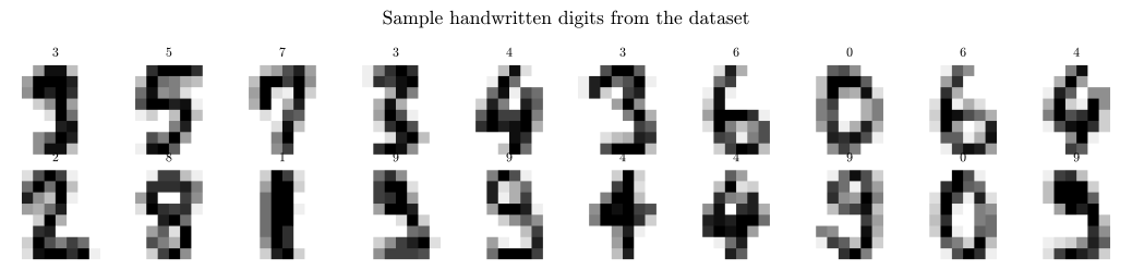
Figure 1: Twenty real examples from the dataset, with their true labels. The handwriting variability is what makes the problem non-trivial despite the small 8×8 resolution.
Step 2: Split into training and test sets before anything else touches the data
from sklearn.model_selection import train_test_split

X_train, X_test, y_train, y_test = train_test_split(
    X, y, test_size=0.2, stratify=y, random_state=42
)
print(f"Train: {X_train.shape[0]}, Test: {X_test.shape[0]}")
Train: 1437, Test: 360
Two details deserve attention, because getting them wrong is among the most common sources of silently inflated results:
-
stratify=yensures the train and test sets preserve the class proportions of the full dataset. Without it, a random split could, by chance, under-represent a digit such as “8” in the training set and degrade the model’s ability to learn it. - The split happens before any preprocessing is fit. Any transformation learned from data, such as the mean and variance of a
StandardScaleror the principal components of aPCA, must be fit only on the training set and then applied to the test set. Fitting preprocessing on the full dataset before splitting leaks test-set information into training. scikit-learn’sPipelineobject (used below) exists largely to make this correct by construction.
Step 3: Baseline models via cross-validation
Instead of selecting one algorithm by instinct, four different model families are compared under identical cross-validation conditions, the same discipline used in the previous post, now applied to a 10-class problem.
from sklearn.model_selection import StratifiedKFold, cross_val_score
from sklearn.preprocessing import StandardScaler
from sklearn.pipeline import Pipeline
from sklearn.linear_model import LogisticRegression
from sklearn.neighbors import KNeighborsClassifier
from sklearn.svm import SVC
from sklearn.ensemble import RandomForestClassifier

models = {
    "Logistic Regression": Pipeline([
        ("scale", StandardScaler()),
        ("clf", LogisticRegression(max_iter=5000, random_state=42)),
    ]),
    "KNN (k=5)": Pipeline([
        ("scale", StandardScaler()),
        ("clf", KNeighborsClassifier(n_neighbors=5)),
    ]),
    "SVM (RBF)": Pipeline([
        ("scale", StandardScaler()),
        ("clf", SVC(kernel="rbf", random_state=42)),
    ]),
    "Random Forest": Pipeline([
        ("clf", RandomForestClassifier(n_estimators=300, random_state=42)),
    ]),
}

cv = StratifiedKFold(n_splits=5, shuffle=True, random_state=42)
for name, pipe in models.items():
    scores = cross_val_score(pipe, X_train, y_train, cv=cv, scoring="accuracy")
    print(f"{name:22s} {scores.mean():.4f} ± {scores.std():.4f}")
5-fold CV accuracy on training set:
Logistic Regression    0.9680 ± 0.0074
KNN (k=5)              0.9756 ± 0.0099
SVM (RBF)              0.9812 ± 0.0061
Random Forest          0.9749 ± 0.0078
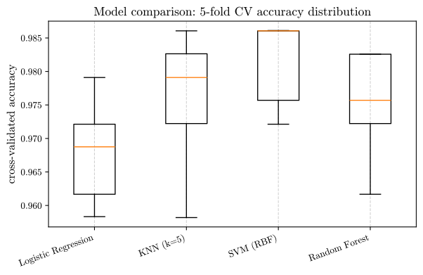
Figure 2: Distribution of 5-fold cross-validation accuracy for each model. The RBF-kernel SVM has both the highest mean accuracy and the tightest spread, which makes it the model worth tuning further.
Unlike the linearly separable breast-cancer data of the previous post, here the RBF-kernel SVM outperforms plain logistic regression. Raw pixel intensities are not linearly separable: a “3” and an “8”, for example, are distinguished by a curved decision boundary, not a hyperplane, and this is the structure a kernel method is designed to capture. That is the purpose of running the comparison instead of assuming an answer: the appropriate model depends on the structure of the data, and that structure differs from one dataset to another.
Step 4: Hyperparameter tuning with GridSearchCV
The SVM’s two key hyperparameters, C (inverse regularization strength) and gamma (kernel bandwidth), are tuned by exhaustive grid search, still using cross-validation so that the test set remains untouched:
from sklearn.model_selection import GridSearchCV

svm_pipe = Pipeline([
    ("scale", StandardScaler()),
    ("clf", SVC(random_state=42)),
])
param_grid = {
    "clf__C": [0.1, 1, 10, 100],
    "clf__gamma": ["scale", 0.001, 0.01, 0.1],
    "clf__kernel": ["rbf"],
}
grid = GridSearchCV(svm_pipe, param_grid, cv=cv, scoring="accuracy", n_jobs=1)
grid.fit(X_train, y_train)
print(f"Best params: {grid.best_params_}")
print(f"Best CV accuracy: {grid.best_score_:.4f}")
Best params: {'clf__C': 1, 'clf__gamma': 'scale', 'clf__kernel': 'rbf'}
Best CV accuracy: 0.9812
The default hyperparameters (C=1, gamma='scale') turned out to be optimal on this grid. This happens more often than newcomers expect, and the search was not wasted: the adequacy of the defaults is established only after checking. Trusting defaults without verification and grid-searching everything indiscriminately are both weaker practices than checking.
Step 5: Visualizing the feature space with PCA
Before finalizing the model, it is useful to see how separable the classes are, using Principal Component Analysis to project the 64-dimensional pixel space onto two dimensions:
from sklearn.decomposition import PCA

pca = PCA(n_components=2, random_state=42)
X_pca = pca.fit_transform(StandardScaler().fit_transform(X))
print(f"First 2 components explain {pca.explained_variance_ratio_.sum()*100:.1f}% of variance")
First 2 components explain 21.6% of variance
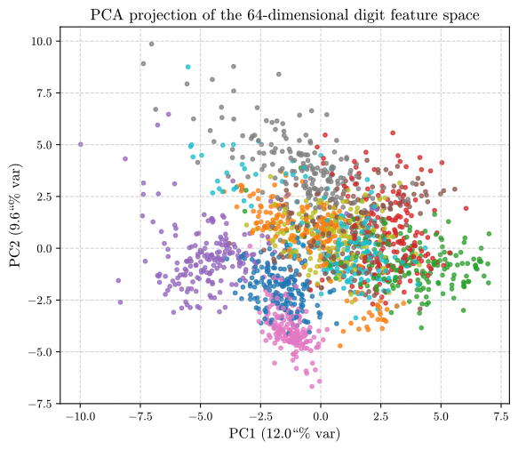
Figure 3: 2D PCA projection of all 1,797 digits, colored by true label. Although these two components capture only 21.6% of the total variance, several digit classes (0, 4, 6) already form visually distinct clusters. This confirms that the problem is learnable, and it indicates why even a linear model, logistic regression, achieved 96.8% above.
Step 6: Learning curves, and whether more data or a better model is required
A learning curve answers a practical question: if this model is underperforming, would more training data help, or is the model itself the bottleneck?
from sklearn.model_selection import learning_curve

train_sizes, train_scores, val_scores = learning_curve(
    grid.best_estimator_, X_train, y_train, cv=cv,
    train_sizes=np.linspace(0.1, 1.0, 8), scoring="accuracy"
)
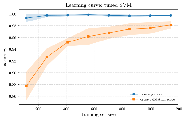
Figure 4: Learning curve for the tuned SVM. The training score (blue) stays high and roughly flat, while the validation score (orange) climbs steadily and the gap between the two curves narrows as more data is added, without fully closing.
A large, persistent gap between the training and validation curves indicates high variance (overfitting), for which more data or stronger regularization would help. Curves that converge to a low plateau indicate high bias (underfitting), which calls for a more flexible model, not more data. Here the gap is narrowing while the validation curve is still climbing at the right edge, which suggests the model has not yet saturated: more training data would likely still help, although with visibly diminishing returns.
Step 7: Final evaluation on the held-out test set
This is the only point at which the test set is used, after every modeling decision has been made by cross-validation alone.
from sklearn.metrics import classification_report, confusion_matrix, accuracy_score

y_pred = grid.best_estimator_.predict(X_test)
test_acc = accuracy_score(y_test, y_pred)
print(f"Final held-out test accuracy: {test_acc:.4f}")
print(classification_report(y_test, y_pred))
Final held-out test accuracy: 0.9750

              precision    recall  f1-score   support
           0       1.00      1.00      1.00        36
           1       0.95      0.97      0.96        36
           2       1.00      1.00      1.00        35
           3       1.00      1.00      1.00        37
           4       0.95      0.97      0.96        36
           5       0.97      1.00      0.99        37
           6       0.97      1.00      0.99        36
           7       0.92      0.97      0.95        36
           8       1.00      0.91      0.96        35
           9       1.00      0.92      0.96        36

    accuracy                           0.97       360
   macro avg       0.98      0.97      0.97       360
weighted avg       0.98      0.97      0.97       360
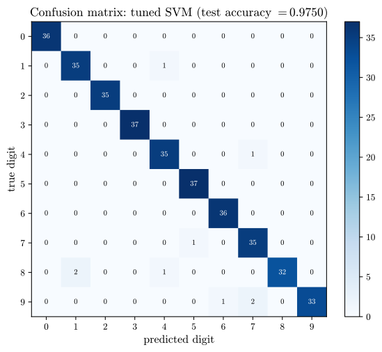
Figure 5: Confusion matrix on the held-out test set. Off-diagonal entries show which digits are confused with which: “9” is occasionally mistaken for “5” or “7”, and “8” for “1”, confusions a human reader might plausibly make as well.

Figure 6: All misclassified test examples (9 out of 360), labeled with True (T) and Predicted (P) digit. Several are ambiguous handwriting even to a human reader, which provides useful context for the 97.5% test accuracy.
scikit-learn: what to take away
- The estimator API (
fit/predict/transform, all composing insidePipeline) is what makes rigorous comparison across models inexpensive: the four-model comparison above takes a few dozen lines because every model exposes the same interface. - Cross-validate before touching the test set, for both model selection and hyperparameter tuning, and never fit preprocessing before splitting. The test set is used exactly once, at the end.
- Examine the individual errors, not only the aggregate metric: the misclassified-digit grid is more diagnostically useful than the 97.5% figure by itself.
Part 2: XGBoost for California Housing Price Prediction
What XGBoost is, and its intended use
XGBoost (“Extreme Gradient Boosting”) is a highly optimized implementation of gradient-boosted decision trees (Chen & Guestrin, 2016), and for several years it was close to the standard winning approach in tabular-data competitions. Compared with scikit-learn’s tree ensembles (Random Forest, Gradient Boosting), XGBoost adds second-order (Newton-style) boosting, explicit L1 and L2 regularization in the training objective, native handling of missing values, and a histogram-based split-finding algorithm that makes it substantially faster on large datasets. The previous post treats these differences mathematically.
The dataset: California Housing
The California Housing dataset (Pace & Barry, 1997) contains 1990 US Census data on median house values across California census block groups, with features including median income, house age, average rooms per household, and geographic coordinates. It replaced the older and ethically problematic Boston Housing dataset as scikit-learn’s standard regression example, and it normally loads with fetch_california_housing(as_frame=True). Because that host was unreachable when the script was run, the script rebuilds the same eight features from the raw census extract distributed with the companion repository of Géron’s Hands-On Machine Learning, dropping the 207 of 20,640 rows with a missing total_bedrooms value:
import numpy as np
import pandas as pd
import xgboost as xgb
from sklearn.model_selection import train_test_split, RandomizedSearchCV, KFold
from sklearn.linear_model import LinearRegression
from sklearn.metrics import root_mean_squared_error, mean_absolute_error, r2_score

df = pd.read_csv(RAW_CSV_PATH)                      # raw census extract (see script)
df = df.dropna(subset=["total_bedrooms"])           # 207/20640 rows dropped (~1%)

X = pd.DataFrame({
    "MedInc": df["median_income"],
    "HouseAge": df["housing_median_age"],
    "AveRooms": df["total_rooms"] / df["households"],
    "AveBedrms": df["total_bedrooms"] / df["households"],
    "Population": df["population"],
    "AveOccup": df["population"] / df["households"],
    "Latitude": df["latitude"],
    "Longitude": df["longitude"],
})
y = df["median_house_value"] / 100_000.0            # match sklearn's $100k units

print(f"Reconstructed dataset: {X.shape[0]} rows, {X.shape[1]} features")
print(X.describe())
print(f"\nTarget (median house value, $100k units): "
      f"mean={y.mean():.2f}, std={y.std():.2f}")
The eight features are MedInc (median income in the block group), HouseAge, AveRooms, AveBedrms, Population, AveOccup, Latitude, and Longitude. After dropping missing values, 20,433 rows remain. This combination of socioeconomic, structural, and geographic features makes a realistic regression problem: noisy, only partially explained by the available features, and with non-linear and geographic interaction effects, since house prices depend on location in ways a linear model captures only crudely.
Step 1: Baseline with a linear model
As in Part 1, a baseline comes first:
X_train, X_test, y_train, y_test = train_test_split(
    X, y, test_size=0.2, random_state=42
)

lr = LinearRegression()
lr.fit(X_train, y_train)
y_pred_lr = lr.predict(X_test)
print(f"Linear Regression  RMSE={root_mean_squared_error(y_test, y_pred_lr):.4f}  "
      f"MAE={mean_absolute_error(y_test, y_pred_lr):.4f}  "
      f"R2={r2_score(y_test, y_pred_lr):.4f}")
Linear Regression RMSE=0.7514 MAE=0.5400 R2=0.5871
The linear model ($R^2 = 0.5871$) captures the broad income-to-price relationship but misses the non-linear, geographic, and interaction effects that account for much of the remaining variance. That gap is what a tree-based model is positioned to close, since trees naturally represent non-linear thresholds and interactions, such as high income combined with coastal latitude, without manual feature engineering.
Step 2: XGBoost with a validation split and early stopping
X_tr, X_val, y_tr, y_val = train_test_split(
    X_train, y_train, test_size=0.2, random_state=42
)

model = xgb.XGBRegressor(
    n_estimators=1000,          # upper bound; early stopping will cut this short
    max_depth=6,
    learning_rate=0.05,
    subsample=0.8,
    colsample_bytree=0.8,
    reg_lambda=1.0,
    reg_alpha=0.0,
    objective="reg:squarederror",
    eval_metric="rmse",
    early_stopping_rounds=30,
    random_state=42,
)

model.fit(
    X_tr, y_tr,
    eval_set=[(X_tr, y_tr), (X_val, y_val)],
    verbose=False,
)

print(f"Best iteration: {model.best_iteration}")
print(f"Best validation RMSE: {model.best_score:.4f}")
Best iteration: 892
Best validation RMSE: 0.4366
XGBoost adds trees one at a time, and each additional tree reduces training error; beyond some point, however, additional trees fit noise in the training set, and validation error stops improving or rises. early_stopping_rounds=30 halts training once the validation metric has not improved for 30 consecutive rounds and keeps the model from the best round. This is a direct practical instance of the bias-variance trade-off.
# Plot train vs validation RMSE across boosting rounds
results = model.evals_result()
epochs = len(results["validation_0"]["rmse"])
fig, ax = plt.subplots(figsize=(7.5, 4.5))
ax.plot(range(epochs), results["validation_0"]["rmse"], label="train")
ax.plot(range(epochs), results["validation_1"]["rmse"], label="validation")
ax.axvline(model.best_iteration, color="gray", linestyle="--",
           label=f"best iteration ({model.best_iteration})")
ax.set_xlabel("boosting round")
ax.set_ylabel("RMSE")
ax.set_title("XGBoost training curve: train vs. validation RMSE")
ax.legend()
savefig_all(fig, "xgb_learning_curve_p6")
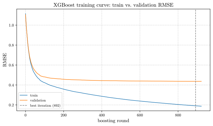
Figure 7: Train and validation RMSE across 922 boosting rounds, with the best iteration (892) marked. The two curves separate progressively after approximately round 100, after which additional trees continue to reduce training error while leaving validation error effectively unchanged.
The training curve decreases smoothly throughout, while the validation curve decreases initially, flattens around round 100, and remains essentially flat out to the best round, 892. Two features of this curve depart from what a textbook description of early stopping would lead one to expect.
First, the gap between the curves is substantial by the end of training. Training RMSE falls to approximately 0.19 while validation RMSE settles near 0.44, a ratio of roughly 2.3. The model has clearly learned structure specific to the training partition. Yet the validation curve does not deteriorate as this gap widens; it flattens and stays flat. The model is fitting training-set noise without that noise corrupting its predictions on unseen data, which is the behavior the subsample=0.8, colsample_bytree=0.8, and reg_lambda=1.0 settings are intended to produce. Removing those settings would be a useful exercise; one would expect the validation curve to begin rising instead of plateauing.
Second, early stopping halted at iteration 892 of a permitted 1000, not at some far earlier round. Given that validation RMSE was essentially flat from round 100 onward, rounds 100 through 892 added negligible accuracy while costing approximately eight times the training time and producing a model roughly eight times larger. The early_stopping_rounds criterion halts when the metric stops improving at all, not when improvement stops being worth its cost. Where inference latency or model size is constrained, a tolerance-based criterion, halting once improvement over a window falls below a threshold, would deliver nearly identical predictive performance at a fraction of the model complexity.
Step 3: Hyperparameter tuning via randomized search
A full grid search over XGBoost’s many hyperparameters is often wasteful. RandomizedSearchCV samples a fixed number of random combinations, which tends to be considerably more efficient in high-dimensional hyperparameter spaces (Bergstra & Bengio, 2012):
from scipy.stats import uniform, randint

param_dist = {
    "max_depth": randint(3, 10),
    "learning_rate": uniform(0.01, 0.29),
    "subsample": uniform(0.6, 0.4),
    "colsample_bytree": uniform(0.6, 0.4),
    "reg_lambda": uniform(0.0, 5.0),
    "reg_alpha": uniform(0.0, 2.0),
}

search = RandomizedSearchCV(
    xgb.XGBRegressor(n_estimators=300, objective="reg:squarederror", random_state=42),
    param_distributions=param_dist,
    n_iter=40,
    cv=KFold(n_splits=5, shuffle=True, random_state=42),
    scoring="neg_root_mean_squared_error",
    random_state=42,
    n_jobs=-1,
)
search.fit(X_train, y_train)
print(f"Best params: {search.best_params_}")
print(f"Best CV RMSE: {-search.best_score_:.4f}")
Best params: {'colsample_bytree': 0.812, 'learning_rate': 0.080,
              'max_depth': 8, 'reg_alpha': 1.794, 'reg_lambda': 4.502,
              'subsample': 0.853}
Best CV RMSE: 0.4445
Step 4: Feature importance and interpretation
The importances below are computed from the early-stopped model of Step 2, not from the tuned model of Step 3:
xgb.plot_importance(model, importance_type="gain", max_num_features=8,
                     title="XGBoost feature importance (gain)")
plt.tight_layout()
savefig_all(fig, "xgb_feature_importance_p6")
XGBoost offers three importance types, and they can disagree substantially:
-
weight: the number of times a feature is used to split across all trees. This measure is biased toward high-cardinality features that offer many possible split points. -
gain: the average improvement in the loss contributed by splits on that feature. This is generally the most informative measure of which features drive predictive power, and it is the one used here. -
cover: the average number of training samples affected by splits on that feature.
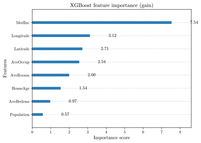
Figure 8: Feature importance by average gain across all trees of the early-stopped model. MedInc dominates, contributing roughly 2.4 times the average gain of the next-ranked feature.
MedInc leads by a wide margin, which is unsurprising given how directly income determines purchasing power. The measured average gains are 7.54 for MedInc, 3.12 for Longitude, 2.71 for Latitude, 2.54 for AveOccup, 2.00 for AveRooms, 1.54 for HouseAge, 0.97 for AveBedrms, and 0.57 for Population. The ordering below the leading feature is more informative than the leader itself.
The geographic coordinates rank second and third, jointly contributing more gain than any single feature other than MedInc. Neither coordinate is meaningful as a predictor on its own; a linear model would extract little from them, since price is not a monotonic function of either. Their value here comes from the ensemble’s ability to partition the coordinate plane into regions and assign a separate price level to each, in effect reconstructing an implicit map of California property markets. Structure of this kind, which a linear functional form cannot represent, plausibly accounts for much of the gap between the linear baseline ($R^2 = 0.5871$) and the tuned ensemble of Step 5 ($R^2 = 0.8509$).
Population ranks last with a gain of 0.57, approximately one-thirteenth that of MedInc. One might expect block-group population to carry information about urban density and therefore price. The likely explanation is redundancy, not irrelevance: AveOccup is population divided by households, so the two features share a numerator, and AveOccup additionally normalizes for household count. Where two features overlap, a boosted ensemble splits preferentially on whichever yields the larger loss reduction, and the gain attributed to the other falls. Low gain therefore means a feature adds little beyond what the other features already supply, which differs from being uninformative in isolation. Discarding Population on this basis would be defensible here, but the same reasoning applied to a feature whose apparent redundancy is an artifact of the particular training sample would not be.
Step 5: Final test-set evaluation
best_model = search.best_estimator_
y_pred = best_model.predict(X_test)
print(f"XGBoost (tuned)  RMSE={root_mean_squared_error(y_test, y_pred):.4f}  "
      f"MAE={mean_absolute_error(y_test, y_pred):.4f}  "
      f"R2={r2_score(y_test, y_pred):.4f}")
XGBoost (tuned) RMSE=0.4515 MAE=0.2918 R2=0.8509
The tuned model reaches $R^2 = 0.8509$ and RMSE $= 0.4515$ (in units of $100,000, a typical error of about $45,000), a substantial improvement over the $R^2 = 0.5871$ of the linear baseline and consistent with the non-linear, interaction-heavy structure discussed above.
XGBoost: what to take away
- Early stopping on a held-out validation set is the standard, automatic guard against overfitting a boosted ensemble. The diagnostic is the validation curve ceasing to improve, or turning upward, while the training curve continues to fall; here it flattened, and early stopping mostly cost training time.
-
RandomizedSearchCVis usually a better use of compute than exhaustive grid search once more than two or three hyperparameters must be tuned together. - Feature importance type matters.
gain,weight, andcovercan give different accounts of the same model, so identify the measure before drawing conclusions.
Part 3: TensorFlow for Handwritten Digit Recognition with a Custom Training Loop
Why this part looks different from the Keras part
Keras is the official high-level API of TensorFlow. To avoid duplicating Part 4, this part uses TensorFlow’s lower-level API: the network’s layers come from tf.keras.layers, but the training loop is written by hand with tf.GradientTape instead of calling model.fit(). This is worth learning even for routine Keras users, because it is what model.fit() does internally, and it becomes necessary whenever a requirement exceeds what the high-level API can express, such as custom losses combining several objectives, non-standard gradient manipulation, or research-style training procedures.
The dataset: MNIST
MNIST (LeCun et al., 1998) comprises 70,000 handwritten digit images (60,000 for training and 10,000 for testing) at 28×28 grayscale pixels, assembled by Yann LeCun and collaborators from NIST handwriting samples. TensorFlow provides a one-line loader; the script instead downloads the original IDX files from a public mirror, for which tf.keras.datasets.mnist.load_data() is a drop-in replacement:
import tensorflow as tf
import numpy as np

(X_train, y_train), (X_test, y_test) = tf.keras.datasets.mnist.load_data()
print(f"Train: {X_train.shape}, Test: {X_test.shape}")   # (60000, 28, 28), (10000, 28, 28)
Train: (60000, 28, 28), Test: (10000, 28, 28)
# Normalize to [0, 1] and add a channel dimension for the convolutional layers
X_train = X_train.astype("float32")[..., None] / 255.0
X_test = X_test.astype("float32")[..., None] / 255.0

# Build a shuffled, batched tf.data pipeline -- TensorFlow's native, efficient
# way to feed data through training, handling batching/shuffling/prefetching
# without materializing the whole shuffled dataset in memory at once.
BATCH_SIZE = 128
train_ds = (
    tf.data.Dataset.from_tensor_slices((X_train, y_train))
    .shuffle(10000)
    .batch(BATCH_SIZE)
    .prefetch(tf.data.AUTOTUNE)
)
test_ds = tf.data.Dataset.from_tensor_slices((X_test, y_test)).batch(BATCH_SIZE)
With 60,000 training images at 28×28 resolution, this is a substantially larger problem than the 1,797 8×8 digits of Part 1, and it is the regime in which the deep learning tools of this and the next two parts begin to justify their additional complexity.
Building a convolutional network from explicit layers
def build_model():
    return tf.keras.Sequential([
        tf.keras.layers.Input(shape=(28, 28, 1)),
        tf.keras.layers.Conv2D(32, 3, activation="relu"),
        tf.keras.layers.MaxPooling2D(2),
        tf.keras.layers.Conv2D(64, 3, activation="relu"),
        tf.keras.layers.MaxPooling2D(2),
        tf.keras.layers.Flatten(),
        tf.keras.layers.Dense(64, activation="relu"),
        tf.keras.layers.Dropout(0.3),
        tf.keras.layers.Dense(10),   # logits, no softmax -- see loss function below
    ])

model = build_model()
Why convolutions, mathematically
A Dense layer connects every input pixel to every output unit with an independent weight: for a 28×28 image, that is 784 weights per unit in the first layer, with no representation of the fact that nearby pixels are related. A convolutional layer instead slides a small shared filter, for example 3×3, across the image, computing
at every spatial location, with the same weights $w_{u,v}$ everywhere. This weight sharing encodes two assumptions that hold for images and that the flattened-pixel approach of Part 1 ignores: locality (nearby pixels are more related than distant ones) and translation equivariance (shifting the input shifts the feature map by the same amount). Pooling then adds approximate translation invariance, so that a “3” remains a “3” whether centered or shifted slightly. These inductive biases are why CNNs substantially outperform flat feedforward networks on image data.
Writing the training loop by hand with GradientTape
In this script the 10,000-image test set is evaluated after every epoch and logged as val_acc. It is therefore test-set monitoring, not a separate validation set; no model selection is done with it here, but the per-epoch figures below should be read with that in mind.
loss_fn = tf.keras.losses.SparseCategoricalCrossentropy(from_logits=True)
optimizer = tf.keras.optimizers.Adam(learning_rate=1e-3)

train_loss_metric = tf.keras.metrics.Mean()
train_acc_metric = tf.keras.metrics.SparseCategoricalAccuracy()
val_acc_metric = tf.keras.metrics.SparseCategoricalAccuracy()

@tf.function   # compiles this function into a TensorFlow graph for speed
def train_step(x_batch, y_batch):
    with tf.GradientTape() as tape:
        logits = model(x_batch, training=True)
        loss = loss_fn(y_batch, logits)
    grads = tape.gradient(loss, model.trainable_variables)
    optimizer.apply_gradients(zip(grads, model.trainable_variables))
    train_loss_metric.update_state(loss)
    train_acc_metric.update_state(y_batch, logits)
    return loss

@tf.function
def val_step(x_batch, y_batch):
    logits = model(x_batch, training=False)
    val_acc_metric.update_state(y_batch, logits)

history = {"train_loss": [], "train_acc": [], "val_acc": []}
EPOCHS = 10
for epoch in range(EPOCHS):
    train_loss_metric.reset_state()
    train_acc_metric.reset_state()
    for x_batch, y_batch in train_ds:
        train_step(x_batch, y_batch)

    val_acc_metric.reset_state()
    for x_batch, y_batch in test_ds:
        val_step(x_batch, y_batch)

    history["train_loss"].append(float(train_loss_metric.result()))
    history["train_acc"].append(float(train_acc_metric.result()))
    history["val_acc"].append(float(val_acc_metric.result()))
    print(f"Epoch {epoch+1}/{EPOCHS}  "
          f"loss={history['train_loss'][-1]:.4f}  "
          f"train_acc={history['train_acc'][-1]:.4f}  "
          f"val_acc={history['val_acc'][-1]:.4f}")
Epoch 1/10   loss=0.2807  train_acc=0.9150  val_acc=0.9819
Epoch 2/10   loss=0.0902  train_acc=0.9733  val_acc=0.9848
Epoch 3/10   loss=0.0664  train_acc=0.9801  val_acc=0.9902
Epoch 4/10   loss=0.0517  train_acc=0.9845  val_acc=0.9908
Epoch 5/10   loss=0.0443  train_acc=0.9862  val_acc=0.9904
Epoch 6/10   loss=0.0376  train_acc=0.9886  val_acc=0.9912
Epoch 7/10   loss=0.0342  train_acc=0.9896  val_acc=0.9911
Epoch 8/10   loss=0.0290  train_acc=0.9908  val_acc=0.9906
Epoch 9/10   loss=0.0267  train_acc=0.9915  val_acc=0.9896
Epoch 10/10  loss=0.0217  train_acc=0.9931  val_acc=0.9915
Each component of this loop does a specific job that model.fit() would otherwise conceal:
-
tf.GradientTape()records every differentiable operation on its watched variables during the forward pass, so thattape.gradient(loss, model.trainable_variables)can compute $\partial \mathcal{L}/\partial \theta$ for every parameter $\theta$ by reverse-mode automatic differentiation: backpropagation, made explicit. -
from_logits=Truetells the loss that the final layer outputs raw, unnormalized scores and that it should apply the numerically stable combined softmax and cross-entropy internally. PyTorch’snn.CrossEntropyLossin Part 5 does the same, for the same reason. -
@tf.functiontraces the Python function once and compiles it into a static graph, which runs considerably faster than eager, line-by-line execution. - Separate
train_acc_metricandval_acc_metricobjects, each reset per epoch, are the idiomatic way to accumulate statistics over atf.datapipeline, so each reports an epoch-level average instead of a noisy single-batch value.
Plotting the training history
fig, axes = plt.subplots(1, 2, figsize=(11, 4.2))
axes[0].plot(history["train_loss"])
axes[0].set_xlabel("epoch"); axes[0].set_ylabel("training loss")
axes[0].set_title("Training loss (sparse categorical cross-entropy)")

axes[1].plot(history["train_acc"], label="train")
axes[1].plot(history["val_acc"], label="validation")
axes[1].set_xlabel("epoch"); axes[1].set_ylabel("accuracy")
axes[1].set_title("Accuracy per epoch")
axes[1].legend()
plt.tight_layout()
savefig_all(fig, "tf_training_curves_p6")
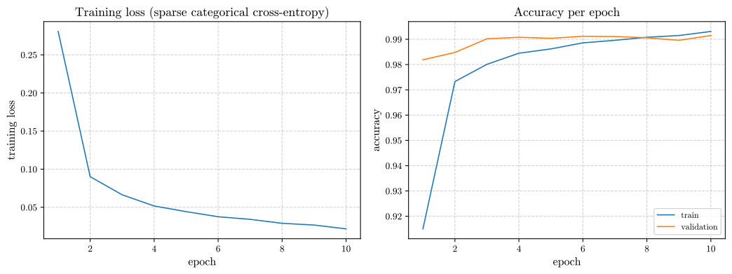
Figure 9: Training loss (left) and per-epoch training and held-out accuracy (right) for the convolutional network on MNIST. The curve labeled “validation” is the test set evaluated each epoch. Held-out accuracy exceeds 98% after a single epoch and improves by less than one percentage point over the remaining nine.
After ten epochs the network reaches 99.31% training and 99.15% held-out accuracy. MNIST is by now close to a solved benchmark, which is why it serves well as a first dataset for learning the mechanics above. The informative quantity is the shape of the curves: training accuracy climbs smoothly across the ten epochs, while held-out accuracy is already high after the first (98.19%) and rises only marginally thereafter. Three aspects of the run bear on how Figure 9 should be read.
Held-out accuracy exceeds training accuracy for the first seven epochs. At epoch 1 the network records 91.50% on the training set against 98.19% on the held-out set. This is neither an error nor a leak. Training accuracy is accumulated during the epoch, averaged over batches while the parameters are still changing, so it includes poor performance on the earliest batches; held-out accuracy is computed after the epoch with the final parameters. Dropout contributes as well: it is active during training (zeroing 30% of the penultimate-layer units) and disabled at evaluation. The curves cross at epoch 8, once the within-epoch parameter change has become small. The same explanation applies to the similar pattern in Part 5.
Held-out accuracy is not monotonic. It peaks at 99.12% (epoch 6), declines to 98.96% (epoch 9), then recovers to 99.15% (epoch 10). These fluctuations span roughly 0.2 percentage points, about 20 images out of 10,000, and reflect the stochasticity of minibatch ordering and dropout, not meaningful differences in model quality. Selecting epoch 6 over epoch 10 on the basis of a 0.03-point difference would attribute meaning to what is, on this evidence, indistinguishable from sampling variation.
Training loss keeps falling while accuracy plateaus. Loss decreases from 0.2807 to 0.0217, more than an order of magnitude, over the same interval in which held-out accuracy improves by less than one percentage point. The network is becoming more confident in predictions that were already correct, since cross-entropy rewards more probability mass on the true class whether or not the argmax was already right. Loss is the quantity being optimized, accuracy is usually the quantity of interest, and the two can diverge substantially.
TensorFlow (low-level API): what to take away
-
GradientTapeis TensorFlow’s explicit automatic-differentiation mechanism; understanding it means understanding what every.fit()call does internally. - Convolutional layers encode locality and translation equivariance directly into the architecture, which is why they outperform flattened-pixel dense networks on images: a better-matched inductive bias, not an opaque gain.
-
from_logits=True, computing softmax and cross-entropy together, is a numerical-stability pattern that recurs across every deep learning framework.
Part 4: Keras for Movie Review Sentiment Classification
Why this part looks different from the TensorFlow part
Part 3 used TensorFlow’s low-level API to show the mechanics; this part presents the other end of the spectrum, the high-level Sequential/fit() workflow of Keras (Chollet & others, 2015), where most everyday deep learning work should be done. The domain also changes, from images to text, to introduce a different kind of architecture: embeddings and recurrent layers instead of convolutions.
The dataset: IMDB Movie Reviews
The IMDB dataset (Maas et al., 2011) consists of 50,000 movie reviews labeled positive or negative, a standard benchmark for binary sentiment classification. Keras ships a pre-tokenized version (keras.datasets.imdb.load_data), but here the script downloads the raw review text from a public CSV mirror and tokenizes it itself, so the whole preprocessing pipeline is visible. It follows the same scheme as the Keras version: a 10,000-word vocabulary of the most frequent words, with indices 0 to 3 reserved for padding, start, unknown, and unused tokens. The reviews are then shuffled and split 25,000/25,000:
import re
import numpy as np
import pandas as pd
from tensorflow import keras

VOCAB_SIZE = 10000     # keep only the 10,000 most frequent words
MAX_LEN = 200          # truncate/pad every review to 200 tokens

df = pd.read_csv(IMDB_CSV_PATH)          # raw IMDB reviews (download in script)

def clean(text):
    text = re.sub(r"<br\s*/?>", " ", text)
    text = re.sub(r"[^a-zA-Z0-9' ]", " ", text)
    return text.lower()

texts = df["review"].apply(clean).tolist()
labels = (df["sentiment"] == "positive").astype(int).values

# Top VOCAB_SIZE words; indices 0-3 reserved for pad/start/unknown/unused.
# Rank words by frequency, ties broken by first appearance (Keras 3 has no
# Tokenizer class, so the vocabulary is built directly).
word_counts = {}
for t in texts:
    for w in t.split():
        word_counts[w] = word_counts.get(w, 0) + 1
ranked = sorted(word_counts, key=lambda w: word_counts[w], reverse=True)
word_index = {w: i + 1 for i, w in enumerate(ranked)}

def encode(text):
    seq = [1]  # <start>
    for w in text.split():
        idx = word_index.get(w)
        seq.append(idx + 3 if (idx is not None and idx < VOCAB_SIZE - 3) else 2)  # 2 = <unk>
    return seq

sequences = [encode(t) for t in texts]

# Standard IMDB-style split: shuffle, then take 25,000/25,000.
rng = np.random.default_rng(42)
perm = rng.permutation(len(sequences))
train_idx, test_idx = perm[:25000], perm[25000:]
X_train_seq = [sequences[i] for i in train_idx]
X_test_seq = [sequences[i] for i in test_idx]
y_train, y_test = labels[train_idx], labels[test_idx]

# Pad/truncate every review to a fixed length so they can be batched into a tensor
X_train = keras.utils.pad_sequences(X_train_seq, maxlen=MAX_LEN)
X_test = keras.utils.pad_sequences(X_test_seq, maxlen=MAX_LEN)

print(f"Train: {len(X_train)} reviews, Test: {len(X_test)} reviews")
print(f"Train label balance: {y_train.mean():.3f} positive")
print(f"Example review (as word indices): {X_train[0][:10]}...")
Train: 25000 reviews, Test: 25000 reviews
Train label balance: 0.498 positive
Example review (as word indices): [   4  372    7    4  176   10  828   18  107 3250]...
The vocabulary is built in plain Python because Keras 3 removed the old keras.preprocessing.text.Tokenizer. keras.layers.TextVectorization is the Keras 3 layer for this job, but it truncates long reviews from the end, whereas the IMDB convention used here keeps the last 200 tokens, so the hand-built version keeps the preprocessing identical. keras.utils.pad_sequences is the Keras 3 location of the padding function, with the same defaults.
Building the model with the Keras Sequential API
model = keras.Sequential([
    keras.layers.Input(shape=(MAX_LEN,)),
    keras.layers.Embedding(input_dim=VOCAB_SIZE, output_dim=32),
    keras.layers.Bidirectional(keras.layers.LSTM(32, return_sequences=False)),
    keras.layers.Dense(32, activation="relu"),
    keras.layers.Dropout(0.4),
    keras.layers.Dense(1, activation="sigmoid"),
])

model.summary()
Two architectural choices are worth understanding:
-
Embedding(VOCAB_SIZE, 32)replaces one-hot encoding of each word (a 10,000-dimensional sparse vector) with a learned, dense 32-dimensional representation. It is a linear projection trained jointly with the rest of the network, which places words that behave similarly for the task near one another. The idea resembles the PCA of Part 1, except that the projection is learned end-to-end for the task instead of fit without supervision to maximize variance. -
Bidirectional(LSTM(32))reads the review forward and backward and concatenates the two representations. An LSTM (Long Short-Term Memory) cell (Hochreiter & Schmidhuber, 1997) maintains an internal memory state, updated at each word by learned gates that control what to retain, forget, and output. It is designed to capture long-range dependencies, such as a negation early in a review reversing the sentiment of praise stated later, which a bag-of-words model would miss.
Compiling and training with model.fit()
Here validation_split=0.2 holds out the last 20% of the training reviews, so the validation figures below come from a genuine validation set, separate from the test set.
model.compile(
    optimizer=keras.optimizers.Adam(learning_rate=1e-3),
    loss="binary_crossentropy",
    metrics=["accuracy"],
)

callbacks = [
    keras.callbacks.EarlyStopping(monitor="val_loss", patience=3, restore_best_weights=True),
    keras.callbacks.ReduceLROnPlateau(monitor="val_loss", factor=0.5, patience=2),
]

history = model.fit(
    X_train, y_train,
    validation_split=0.2,
    epochs=20,
    batch_size=64,
    callbacks=callbacks,
    verbose=1,
)
Epoch 1/20  loss=0.4893 acc=0.7541 val_loss=0.3394 val_acc=0.8630
Epoch 2/20  loss=0.2718 acc=0.8940 val_loss=0.2996 val_acc=0.8742  (best epoch)
Epoch 3/20  loss=0.2164 acc=0.9184 val_loss=0.3214 val_acc=0.8720
Epoch 4/20  loss=0.1916 acc=0.9291 val_loss=0.3685 val_acc=0.8686  (LR reduced after this epoch: 1e-3 -> 5e-4)
Epoch 5/20  loss=0.1234 acc=0.9567 val_loss=0.4299 val_acc=0.8756
Training halted by early stopping (patience=3); weights restored from epoch 2
Validation loss reaches its minimum at epoch 2. With patience=2, ReduceLROnPlateau halves the learning rate after two non-improving epochs, that is, at the end of epoch 4, and EarlyStopping halts after three, at the end of epoch 5, restoring the epoch-2 weights.
This single call replaces the entire training loop of Part 3: the GradientTape block, the manual metric tracking, and the epoch loop. That compression is the value proposition of Keras: most supervised deep learning problems need no custom gradient logic, and hiding that boilerplate behind .fit() leaves fewer places for bugs. Two callbacks deserve comment:
-
ReduceLROnPlateaushrinks the learning rate when validation loss stops improving, a simple adaptive schedule that lets the optimizer take large steps early and smaller ones later without a hand-tuned decay schedule. -
EarlyStopping(restore_best_weights=True)is the neural-network analog of XGBoost’searly_stopping_roundsin Part 2: the same purpose, the same mechanism (monitoring validation performance), and an entirely different model class.
Plotting and interpreting the training curves
fig, axes = plt.subplots(1, 2, figsize=(11, 4.2))
axes[0].plot(history.history["loss"], label="train")
axes[0].plot(history.history["val_loss"], label="validation")
axes[0].set_xlabel("epoch"); axes[0].set_ylabel("loss")
axes[0].set_title("Binary cross-entropy loss")
axes[0].legend()

axes[1].plot(history.history["accuracy"], label="train")
axes[1].plot(history.history["val_accuracy"], label="validation")
axes[1].set_xlabel("epoch"); axes[1].set_ylabel("accuracy")
axes[1].set_title("Classification accuracy")
axes[1].legend()
plt.tight_layout()
savefig_all(fig, "keras_training_curves_p6")

test_loss, test_acc = model.evaluate(X_test, y_test, verbose=0)
print(f"Test accuracy: {test_acc:.4f}, test loss: {test_loss:.4f}")
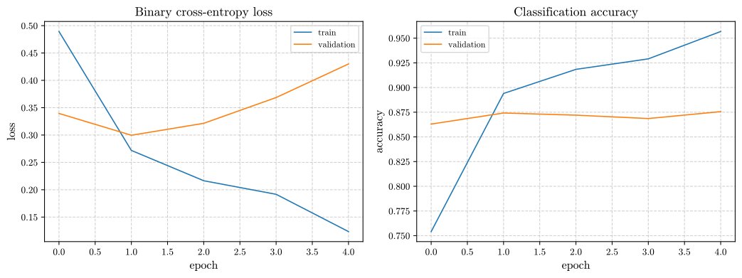
Figure 10: Binary cross-entropy loss (left) and classification accuracy (right) for the bidirectional LSTM over the five epochs run. Validation loss reaches its minimum at epoch 2 and rises thereafter, while training loss continues to fall.
Test accuracy: 0.8733, test loss: 0.2986
The restored epoch-2 model reaches 87.33% test accuracy. That is respectable, though below what modern transformer-based models (Vaswani et al., 2017) achieve on the same task, which reflects the limitations of recurrent models on long-range text dependencies relative to attention-based approaches.
This run is the most instructive of the four for a reason unrelated to its accuracy: it is the only one in which overfitting is unambiguous.
Validation loss rises while validation accuracy does not fall. Between epochs 2 and 5, validation loss increases from 0.2996 to 0.4299, roughly 43%, while validation accuracy stays in a narrow band between 86.86% and 87.56%, ending slightly higher than at epoch 2. The additional training changed less which reviews the model classifies correctly than how confidently it commits to its predictions. Because cross-entropy penalizes confident errors far more heavily than tentative ones, a model growing more certain about a fixed set of mistakes shows sharply rising loss with essentially unchanged accuracy. This is why EarlyStopping monitors val_loss here: loss registered the degradation from epoch 3 onward, while accuracy barely moved over the five epochs run.
The reduced learning rate did not arrest the divergence. ReduceLROnPlateau halved the learning rate from $10^{-3}$ to $5 \times 10^{-4}$ after epoch 4, and validation loss nonetheless rose further at epoch 5. A smaller step size lets the optimizer settle more precisely into a minimum it is approaching; it does not stop the optimizer from converging toward a minimum of the training objective that differs from the minimum of the generalization error. The model was not oscillating around a good solution, the pathology a schedule addresses; it was converging accurately toward an overfit one.
Training accuracy reaches 95.67% against a validation ceiling near 87.6%. The gap of about eight percentage points by epoch 5 quantifies how much of the training set the model has memorized instead of generalized from. With a 10,000-word vocabulary embedded in 32 dimensions and 25,000 training reviews, a model of this capacity can easily memorize idiosyncrasies of individual reviews. Dropout(0.4) and early stopping oppose this, and early stopping did most of the work here, since dropout alone did not prevent training accuracy from climbing steeply after epoch 2.
These observations qualify the headline figure. The 87.33% is the test accuracy of the epoch-2 model, recovered by restore_best_weights=True. Without that setting, the reported figure would have come from the epoch-5 weights, with 43% higher validation loss and worse calibration at roughly the same accuracy, and the headline metric would have concealed the difference almost entirely.
Evaluating on new text
def predict_sentiment(text, tokenizer_word_index=word_index):
    tokens = text.lower().split()
    encoded = [1] + [
        (tokenizer_word_index.get(w) + 3)
        if (tokenizer_word_index.get(w) is not None and tokenizer_word_index.get(w) < VOCAB_SIZE - 3)
        else 2
        for w in tokens
    ]
    padded = keras.utils.pad_sequences([encoded], maxlen=MAX_LEN)
    prob = model.predict(padded, verbose=0)[0, 0]
    return ("positive" if prob > 0.5 else "negative"), prob

sentiment, prob = predict_sentiment("this movie was a genuine waste of time")
print(f"Predicted: {sentiment} (p={prob:.3f})")
Predicted: negative (p=0.085)
A second, oppositely valenced example, “an absolutely brilliant and moving film”, was classified as positive with p=0.907. Both hand-written examples were classified correctly, with probabilities well away from the decision boundary.
Testing on hand-written examples is sound practice for probing failure modes the test distribution may not surface, such as sarcasm, mixed sentiment, or words outside the 10,000-word vocabulary. The fallback to index 2 maps such words to the <unk> token and silently discards their information, a real limitation of this preprocessing pipeline.
Keras: what to take away
-
model.fit()does everything theGradientTapeloop of Part 3 does explicitly; the benefit is fewer lines and fewer opportunities for bugs, not different mathematics. - Recurrent architectures such as the LSTM exist to capture order-dependent, long-range structure in sequences, but attention-based (transformer) models generally outperform them on this class of task.
- Callbacks (
EarlyStopping,ReduceLROnPlateau) inject training-loop logic without a manual loop. Learn the built-in ones before writing a custom loop for behavior a callback probably already covers.
Part 5: PyTorch for Clothing Image Classification with a Custom CNN
What PyTorch is, and how it differs philosophically
PyTorch’s (Paszke et al., 2019) defining design choice is imperative, eager execution: every operation runs immediately, as plain Python/NumPy code would, and the computational graph used for backpropagation is built dynamically on each forward pass. This distinguishes it from the declarative Sequential style of Keras and makes it well suited to architectures with data-dependent control flow, such as a variable number of layers depending on the input, recursive structures, or custom training procedures, which accounts in large part for its prevalence in research code.
The dataset: Fashion-MNIST
Fashion-MNIST (Xiao et al., 2017) is a drop-in replacement for MNIST: 70,000 28×28 grayscale images of clothing items (t-shirts, trousers, shoes, bags, and similar) in 10 categories, built by Zalando Research because plain MNIST had become too easy to differentiate modern methods. It ships in torchvision; the script downloads the same IDX files from Zalando Research’s own repository, for which the torchvision loader below is a drop-in replacement:
import torch
import torch.nn as nn
import torch.optim as optim
from torch.utils.data import DataLoader
import torchvision
import torchvision.transforms as transforms

device = torch.device("cuda" if torch.cuda.is_available() else "cpu")
print(f"Using device: {device}")

transform = transforms.Compose([
    transforms.ToTensor(),                       # scales pixels to [0, 1]
    transforms.Normalize((0.5,), (0.5,)),         # rescale to roughly [-1, 1]
])

train_set = torchvision.datasets.FashionMNIST(
    root="./data", train=True, download=True, transform=transform
)
test_set = torchvision.datasets.FashionMNIST(
    root="./data", train=False, download=True, transform=transform
)

class_names = ["T-shirt/top", "Trouser", "Pullover", "Dress", "Coat",
               "Sandal", "Shirt", "Sneaker", "Bag", "Ankle boot"]

train_loader = DataLoader(train_set, batch_size=128, shuffle=True, num_workers=2)
test_loader = DataLoader(test_set, batch_size=256, shuffle=False, num_workers=2)

print(f"Train: {len(train_set)}, Test: {len(test_set)}")
Using device: cpu
Train: 60000, Test: 10000
DataLoader is PyTorch’s counterpart to the tf.data.Dataset pipeline of Part 3. It handles batching, shuffling, and, through num_workers, parallel loading in background processes, so the device doing the training rarely waits for the next batch.
Defining the network as an nn.Module subclass
class FashionCNN(nn.Module):
    def __init__(self):
        super().__init__()
        self.conv_block = nn.Sequential(
            nn.Conv2d(1, 32, kernel_size=3, padding=1),
            nn.ReLU(),
            nn.MaxPool2d(2),                      # 28x28 -> 14x14
            nn.Conv2d(32, 64, kernel_size=3, padding=1),
            nn.ReLU(),
            nn.MaxPool2d(2),                      # 14x14 -> 7x7
        )
        self.classifier = nn.Sequential(
            nn.Flatten(),
            nn.Linear(64 * 7 * 7, 128),
            nn.ReLU(),
            nn.Dropout(0.3),
            nn.Linear(128, 10),                   # logits over 10 classes
        )

    def forward(self, x):
        x = self.conv_block(x)
        return self.classifier(x)

model = FashionCNN().to(device)
print(model)
This network has the same overall structure as the TensorFlow CNN of Part 3, two convolution-and-pooling blocks followed by a dense head with dropout, but the two are not identical: here the convolutions use padding=1, so each pooling step halves the spatial size exactly (28 to 14 to 7), and the hidden dense layer has 128 units, whereas the TensorFlow model uses unpadded convolutions and a 64-unit hidden layer. The broader point stands: the mathematical model is framework-agnostic, and what differs between frameworks is the surrounding machinery (data pipelines, training loop, deployment path).
The training loop, written explicitly (PyTorch’s default style)
As in Part 3, the test set is evaluated after every epoch (logged here, accurately, as test_acc); it is monitored but not used for any training decision.
criterion = nn.CrossEntropyLoss()   # combines log-softmax + NLL loss internally
optimizer = optim.Adam(model.parameters(), lr=1e-3)
scheduler = optim.lr_scheduler.StepLR(optimizer, step_size=5, gamma=0.5)

def train_one_epoch():
    model.train()
    running_loss, correct, total = 0.0, 0, 0
    for images, labels in train_loader:
        images, labels = images.to(device), labels.to(device)

        optimizer.zero_grad()
        outputs = model(images)
        loss = criterion(outputs, labels)
        loss.backward()
        optimizer.step()

        running_loss += loss.item() * images.size(0)
        correct += (outputs.argmax(dim=1) == labels).sum().item()
        total += labels.size(0)
    return running_loss / total, correct / total

@torch.no_grad()
def evaluate(loader):
    model.eval()
    correct, total = 0, 0
    for images, labels in loader:
        images, labels = images.to(device), labels.to(device)
        outputs = model(images)
        correct += (outputs.argmax(dim=1) == labels).sum().item()
        total += labels.size(0)
    return correct / total

EPOCHS = 10
history = {"train_loss": [], "train_acc": [], "test_acc": []}
for epoch in range(EPOCHS):
    train_loss, train_acc = train_one_epoch()
    test_acc = evaluate(test_loader)
    scheduler.step()

    history["train_loss"].append(train_loss)
    history["train_acc"].append(train_acc)
    history["test_acc"].append(test_acc)
    print(f"Epoch {epoch+1}/{EPOCHS}  loss={train_loss:.4f}  "
          f"train_acc={train_acc:.4f}  test_acc={test_acc:.4f}  "
          f"lr={scheduler.get_last_lr()[0]:.5f}")
Epoch 1/10   loss=0.5247  train_acc=0.8089  test_acc=0.8656  lr=0.00100
Epoch 2/10   loss=0.3314  train_acc=0.8800  test_acc=0.8886  lr=0.00100
Epoch 3/10   loss=0.2818  train_acc=0.8970  test_acc=0.9002  lr=0.00100
Epoch 4/10   loss=0.2479  train_acc=0.9092  test_acc=0.9094  lr=0.00100
Epoch 5/10   loss=0.2240  train_acc=0.9174  test_acc=0.9114  lr=0.00050
Epoch 6/10   loss=0.1901  train_acc=0.9298  test_acc=0.9175  lr=0.00050
Epoch 7/10   loss=0.1781  train_acc=0.9351  test_acc=0.9216  lr=0.00050
Epoch 8/10   loss=0.1661  train_acc=0.9387  test_acc=0.9224  lr=0.00050
Epoch 9/10   loss=0.1551  train_acc=0.9423  test_acc=0.9247  lr=0.00050
Epoch 10/10  loss=0.1446  train_acc=0.9468  test_acc=0.9240  lr=0.00025
This pattern, or a close variant, is what almost every PyTorch training script looks like, and each line is deliberate:
-
optimizer.zero_grad()must be called before each backward pass, because PyTorch accumulates gradients into.gradby default. This supports techniques such as gradient accumulation across memory-constrained mini-batches, but it silently corrupts training if the reset is omitted. -
loss.backward()runs reverse-mode automatic differentiation through the graph built during this forward pass, populating.gradon every parameter: the PyTorch equivalent oftape.gradient(...)in Part 3. -
@torch.no_grad()onevaluate()disables gradient tracking during inference, reducing memory use and speeding up the forward pass. -
model.train()/model.eval()toggle layer-specific behavior.Dropoutis active in.train()and passes data through unchanged in.eval();BatchNormlayers (not used here) switch between batch statistics and stored running statistics. Forgetting.eval()before evaluation is one of the most common and hardest-to-notice PyTorch bugs, since the model still produces plausible but silently degraded predictions. -
StepLRhalves the learning rate every 5 epochs: a fixed schedule, whereReduceLROnPlateauin Part 4 reacts to validation performance.
Plotting results and inspecting predictions
fig, axes = plt.subplots(1, 2, figsize=(11, 4.2))
axes[0].plot(history["train_loss"])
axes[0].set_xlabel("epoch"); axes[0].set_ylabel("training loss")
axes[0].set_title("Training loss")

axes[1].plot(history["train_acc"], label="train")
axes[1].plot(history["test_acc"], label="test")
axes[1].set_xlabel("epoch"); axes[1].set_ylabel("accuracy")
axes[1].set_title("Accuracy per epoch")
axes[1].legend()
plt.tight_layout()
savefig_all(fig, "pytorch_training_curves_p6")

# Visualize a batch of predictions
model.eval()
images, labels = next(iter(test_loader))
with torch.no_grad():
    preds = model(images.to(device)).argmax(dim=1).cpu()

fig, axes = plt.subplots(2, 8, figsize=(14, 4))
for ax, img, true, pred in zip(axes.ravel(), images[:16], labels[:16], preds[:16]):
    ax.imshow(img.squeeze(), cmap="gray")
    color = "green" if true == pred else "red"
    ax.set_title(f"{class_names[pred]}", fontsize=8, color=color)
    ax.axis("off")
fig.suptitle("Predictions (green=correct, red=incorrect)")
plt.tight_layout()
savefig_all(fig, "pytorch_predictions_p6")
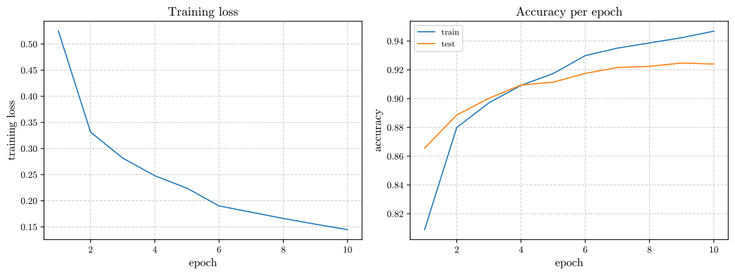
Figure 11: Training loss (left) and per-epoch training and test accuracy (right) for the convolutional network on Fashion-MNIST. The two accuracy curves cross at approximately epoch 4, after which training accuracy advances more rapidly than test accuracy.
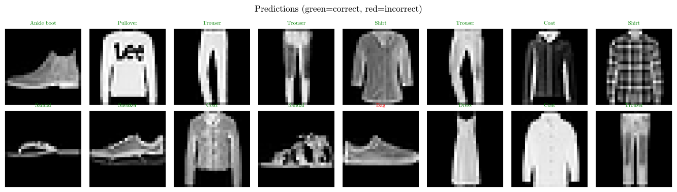
Figure 12: Predictions on the first sixteen test images, correct in green and incorrect in red. Fifteen of the sixteen are classified correctly; the single error is a sneaker assigned to the “Bag” class.
The network reaches 92.40% test accuracy after 10 epochs. The task is harder than MNIST, on which the similar network of Part 3 reached 99.15%, since categories such as “shirt”, “pullover”, and “coat” are visually ambiguous at low grayscale resolution. By the final epoch, training accuracy (94.68%) has drawn visibly ahead of test accuracy.
The accuracy curves cross, and the crossing point is informative. For the first three epochs test accuracy exceeds training accuracy, for the reasons given in Part 3. The curves meet at approximately epoch 4, and the gap then widens in the opposite direction, reaching 2.28 percentage points by epoch 10. On MNIST the curves crossed only at epoch 8 and separated by roughly 0.16 points. With similar architectures, the same optimizer, and the same number of epochs, the gap on Fashion-MNIST is about an order of magnitude larger. A plausible reading is that where the generalizable signal is weaker, a fixed-capacity model devotes more of its capacity to memorization, although the two networks are not identical and this single comparison cannot isolate the cause.
Test accuracy peaks at epoch 9, not epoch 10. The final epoch records 92.40% against 92.47% at epoch 9, a decline of 0.07 points, roughly 7 images out of 10,000, which should not be over-interpreted. The detail matters mainly because this run has no early-stopping mechanism: the loop runs ten epochs and reports whatever state it reaches. Over a longer run, nothing in this script would detect or halt a widening gap; the Keras callbacks of Part 4 supply exactly that.
The learning-rate schedule had a visible effect. StepLR halved the learning rate after epoch 5 and again after epoch 10. Between epochs 5 and 6, immediately after the first reduction, test accuracy rose by 0.61 points, three times the 0.20-point gain of the preceding epoch (larger gains occurred only early in training: 2.30 points from epoch 1 to 2 and 1.16 from epoch 2 to 3). Training loss fell by 0.034 over the same interval, against 0.024 in the preceding one. This is the behavior a schedule is intended to produce, and it contrasts with Part 4, where the reduction came after overfitting had begun and did not help. Reducing the step size while the model is still improving allows finer convergence; reducing it after generalization has begun to degrade merely refines the descent toward an overfit solution.
The individual errors are semantically plausible. In Figure 12, the single misclassification assigns a sneaker to the “Bag” class. At 28×28 grayscale resolution, a low side-on shoe and a flat handbag share a broadly similar outline, and the distinguishing evidence (a sole, laces, a strap) occupies few pixels. As in Part 1, inspecting the errors distinguishes a model that has failed to learn the task from one meeting the limits of its input representation. These errors look like the latter, which suggests that improving on 92.40% would require higher-resolution inputs or data augmentation more than a larger network.
PyTorch: what to take away
- Eager execution means PyTorch code can be debugged with standard Python tools (
print, a debugger, stepping line by line), without a separate graph-compilation step such as@tf.function. -
optimizer.zero_grad()before every backward pass is not boilerplate to skim: omitting it silently accumulates gradients across steps. -
model.train()/model.eval()change model behavior through dropout and batch normalization. Call.eval()before evaluation or inference and.train()before resuming training.
What the four runs show when read together
Several patterns across Parts 2 to 5 become visible only in comparison.
| Section | Task | Measured result | Overfitting gap |
|---|---|---|---|
| Part 2: XGBoost | California Housing regression | $R^2 = 0.8509$, RMSE $= 0.4515$ | Train RMSE 0.19 vs. validation 0.44 |
| Part 3: TensorFlow | MNIST digit classification | 99.15% held-out (test-set) accuracy | 0.16 points |
| Part 4: Keras | IMDB sentiment classification | 87.33% test accuracy | ≈8 points |
| Part 5: PyTorch | Fashion-MNIST classification | 92.40% test accuracy | 2.28 points |
The size of the overfitting gap varied widely across the deep-learning runs. The three deep-learning parts use comparable regularization (dropout at 0.3 to 0.4) and the same optimizer (Adam (Kingma & Ba, 2015) at $10^{-3}$), yet the train-test gap spans two orders of magnitude: 0.16 points on MNIST, 2.28 on Fashion-MNIST, and approximately 10 on IMDB. This ordering matches the intuitive difficulty of the three tasks, which is consistent with the idea that a model memorizes more when generalizable structure is scarce relative to its capacity. The comparison is confounded, however: the architectures, data modalities, and dataset sizes all differ, so it is an observation, not evidence that task difficulty alone drives the gap. A practical corollary is still useful: whether a train-test gap exists matters less than whether it is proportionate to the difficulty of what is being learned.
Loss and accuracy (or training and validation error) diverged in every run, and monitoring the wrong one has consequences. In Part 2, validation RMSE flattened while training RMSE continued to fall. In Part 3, training loss fell by an order of magnitude while held-out accuracy moved by less than one percentage point. In Part 4, validation loss rose by 43% while validation accuracy remained essentially constant. Loss is the quantity being optimized and responds to changes in confidence; accuracy is typically the quantity of interest and responds only to changes in the argmax. In Part 4, val_loss exposed the degradation clearly while val_accuracy barely moved, which is why the early-stopping callback monitors loss.
Early stopping was decisive in one of the four runs and inconsequential in the others. The XGBoost run halted at iteration 892 of 1000, long after the validation curve had flattened, which cost training time without affecting accuracy. The Keras run halted at epoch 5 of 20 and restored the epoch-2 weights, which materially changed the reported model. The TensorFlow and PyTorch runs had no early-stopping mechanism and simply completed ten epochs. Early stopping is essential when the validation metric deteriorates and largely decorative when it merely plateaus.
Choosing among the four libraries: an updated decision framework
Having built a complete pipeline in each library, the guidance of the previous post holds, now with more detail attached to each row:
| Situation | Recommended tool | Rationale (from the implementations above) |
|---|---|---|
| Small-to-medium tabular data, need interpretability | scikit-learn | Pipeline + cross-validation + model comparison is a few dozen lines, and the digit-classification example showed even a linear baseline can be competitive |
| Larger tabular data, need best-in-class accuracy with less tuning effort | XGBoost | Second-order boosting + built-in regularization + early stopping closed a real, measurable gap over a linear baseline on California Housing |
| Image, audio, or other spatial/grid-structured data | TensorFlow or PyTorch (CNNs) | Convolutional weight sharing encodes locality and translation equivariance directly; a flattened-pixel Dense/Linear layer cannot match this without far more data |
| Sequential/text data with long-range dependencies | Keras/TensorFlow or PyTorch (RNNs, or better, attention-based models) | The LSTM learned useful sentiment structure on IMDB, though with a clear accuracy ceiling relative to modern transformer architectures |
| Need to iterate quickly on standard architectures | Keras Sequential/fit() | Model definition, callbacks, and training for IMDB fit in a few dozen lines |
| Need custom training logic, research-style flexibility | PyTorch, or TensorFlow’s low-level GradientTape API | Both expose the backward-pass and optimizer-step mechanics directly, at the cost of writing more boilerplate yourself |
| Deploying to production, mobile, or edge devices | TensorFlow (TF Lite, TF Serving) | Not demonstrated above, but an ecosystem advantage worth knowing about when a project reaches that stage |
Summary
- The underlying mathematics is shared far more than the different APIs suggest. Gradient-based optimization, regularization, and early stopping appear, in some form, in every part. A boosted tree ensemble and a bidirectional LSTM address the same kind of problem, minimizing a loss without overfitting the training set, with very different function classes.
- Start with a baseline. Every part began with a baseline or a comparison of simple models before adopting a more sophisticated tool. The baseline is not always the winner: in Part 1 the RBF-kernel SVM (0.9812 cross-validated accuracy) beat logistic regression (0.9680), and in Part 2 XGBoost raised $R^2$ from 0.5871 to 0.8509. The value of the baseline is that it measures how much the extra complexity buys.
- Validation curves are the most repeated diagnostic. Cross-validation in scikit-learn, the train/validation RMSE plot in XGBoost, and the per-epoch curves in the deep-learning parts all perform the same check: whether the model is learning generalizable structure or memorizing the training set.
- Framework choice is an engineering decision, not a modeling one. Once a CNN is needed, the choice between TensorFlow and PyTorch has little effect on what the model can learn; it is a question of ecosystem fit, deployment target, team familiarity, and the relative value of declarative concision (Keras) and explicit control (PyTorch and low-level TensorFlow).
References
The scikit-learn ecosystem used in Part 1 is documented in (Pedregosa et al., 2011), with the digits dataset from (Alpaydin & Kaynak, 1998). The California Housing dataset used in Part 2 originates with (Pace & Barry, 1997), and the XGBoost algorithm follows (Chen & Guestrin, 2016), with the randomized-search strategy supported by (Bergstra & Bengio, 2012). The MNIST dataset and CNN architecture in Part 3 trace back to (LeCun et al., 1998), built on TensorFlow (Abadi Martı́n et al., 2016). The IMDB sentiment dataset in Part 4 is from (Maas et al., 2011); the LSTM architecture used there follows (Hochreiter & Schmidhuber, 1997), with (Vaswani et al., 2017) noted as the modern successor architecture, and Keras documented in (Chollet & others, 2015). The Fashion-MNIST dataset used in Part 5 is from (Xiao et al., 2017), built on PyTorch (Paszke et al., 2019). The Adam optimizer (Kingma & Ba, 2015) and dropout regularization (Srivastava et al., 2014) recur across every deep-learning part.
- Alpaydin, E., & Kaynak, C. (1998). Optical Recognition of Handwritten Digits Data Set. UCI Machine Learning Repository.
- Chen, T., & Guestrin, C. (2016). XGBoost: A Scalable Tree Boosting System. Proceedings of the 22nd ACM SIGKDD International Conference on Knowledge Discovery and Data Mining, 785–794.
- Pace, R. K., & Barry, R. (1997). Sparse Spatial Autoregressions. Statistics & Probability Letters, 33(3), 291–297.
- Bergstra, J., & Bengio, Y. (2012). Random Search for Hyper-Parameter Optimization. Journal of Machine Learning Research, 13, 281–305.
- LeCun, Y., Bottou, L., Bengio, Y., & Haffner, P. (1998). Gradient-Based Learning Applied to Document Recognition. Proceedings of the IEEE, 86(11), 2278–2324.
- Chollet, F., & others. (2015). Keras. https://keras.io
- Maas, A. L., Daly, R. E., Pham, P. T., Huang, D., Ng, A. Y., & Potts, C. (2011). Learning Word Vectors for Sentiment Analysis. Proceedings of the 49th Annual Meeting of the Association for Computational Linguistics (ACL), 142–150.
- Hochreiter, S., & Schmidhuber, J. (1997). Long Short-Term Memory. Neural Computation, 9(8), 1735–1780.
- Vaswani, A., Shazeer, N., Parmar, N., Uszkoreit, J., Jones, L., Gomez, A. N., Kaiser, Ł., & Polosukhin, I. (2017). Attention Is All You Need. Advances in Neural Information Processing Systems (NeurIPS), 30.
- Paszke, A., Gross, S., Massa, F., Lerer, A., Bradbury, J., Chanan, G., Killeen, T., Lin, Z., Gimelshein, N., Antiga, L., & others. (2019). PyTorch: An Imperative Style, High-Performance Deep Learning Library. Advances in Neural Information Processing Systems (NeurIPS), 32, 8026–8037.
- Xiao, H., Rasul, K., & Vollgraf, R. (2017). Fashion-MNIST: A Novel Image Dataset for Benchmarking Machine Learning Algorithms. ArXiv Preprint ArXiv:1708.07747.
- Kingma, D. P., & Ba, J. (2015). Adam: A Method for Stochastic Optimization. 3rd International Conference on Learning Representations (ICLR).
- Pedregosa, F., Varoquaux, G., Gramfort, A., Michel, V., Thirion, B., Grisel, O., Blondel, M., Prettenhofer, P., Weiss, R., Dubourg, V., & others. (2011). Scikit-Learn: Machine Learning in Python. Journal of Machine Learning Research, 12, 2825–2830.
- Abadi Martı́n, Barham, P., Chen, J., Chen, Z., Davis, A., Dean, J., Devin, M., Ghemawat, S., Irving, G., Isard, M., & others. (2016). TensorFlow: A System for Large-Scale Machine Learning. 12th USENIX Symposium on Operating Systems Design and Implementation (OSDI 16), 265–283.
- Srivastava, N., Hinton, G., Krizhevsky, A., Sutskever, I., & Salakhutdinov, R. (2014). Dropout: A Simple Way to Prevent Neural Networks from Overfitting. Journal of Machine Learning Research, 15(1), 1929–1958.
Full, executed code for each part is available as a self-contained script: sklearn_digits_tutorial_p6.py (Part 1), xgboost_california_housing_p6.py (Part 2), tensorflow_mnist_p6.py (Part 3), keras_imdb_sentiment_p6.py (Part 4), and pytorch_fashion_mnist_p6.py (Part 5). Each script retrieves its own data and runs end to end, and every number, table, and figure in this post was produced by an actual run.