Motivation
Third-order spatial derivatives appear in every dispersive wave model, of which the Korteweg-de Vries (KdV) equation is the canonical example. Their accurate approximation matters well beyond KdV itself: the same third-derivative operators arise in Airy-type dispersion terms for internal waves, in certain regularized shock-capturing schemes, and in the dispersive-error budgets that govern long-time wave propagation generally.
Classical compact (Padé-type) schemes, following Lele (Lele, 1992), obtain spectral-like resolution from narrow stencils at the cost of a matrix inversion at each evaluation. Node-based compact schemes are accurate but lose resolution at short wavelengths. Cell-centered compact schemes improve resolution but require an interpolation step onto the staggered grid, and that interpolation introduces transfer errors which offset part of the resolution gain.
This post reproduces, derives, and validates the scheme proposed by Salian, Samala, and Ghosh (Salian et al., 2026), published in Numerical Methods for Partial Differential Equations (2026, 42:e70060). The paper is openly available from the author’s website, through the publications page or as a direct PDF. Its contribution is a third option: retain both the node values and the cell-center values as independently evolved variables, and compute derivatives at each set of points using values from both grids, with no interpolation at any stage. The authors designate this the third-derivative central compact scheme (TDCCS).
The original work uses MATLAB, and its code is not publicly available. The implementation presented here is therefore an open-source alternative, intended also as an entry point for readers approaching compact finite differences for the first time.
Three objectives structure what follows: to derive the coefficients of the scheme instead of transcribing the published tables, to implement the scheme and verify it against the paper’s own reported values, and to state explicitly where the reproduction is exact and where it necessarily diverges. The third objective is not incidental. Four of the paper’s six numerical examples use first-derivative operators cited from other sources but not written out numerically in the paper itself, so any independent reproduction encounters the difficulty documented in Section 4 below.
1. The three schemes and the basis of comparison
All three schemes approximate $f’’’$ at the same order of accuracy, from a pentadiagonal (or tridiagonal, or explicit) implicit relation of the form
\[\beta f'''_{j-2} + \alpha f'''_{j-1} + f'''_j + \alpha f'''_{j+1} + \beta f'''_{j+2} = \text{(explicit combination of } f \text{ values)}.\]They differ only in the grid from which the explicit right-hand side draws its values:
| Scheme | RHS uses values at | Requires interpolation |
|---|---|---|
| TDCNCS (node-based, Eq. 2.4) | nodes only | no |
| TDCCCS (cell-centered, Eq. 2.5) | cell centers only | yes, to obtain the centers |
| TDCCS (the paper’s new scheme, Eq. 3.1-3.2) | both nodes and centers, evolved together | no |
The principle underlying TDCCS is simple once stated. TDCCCS interpolates $f$ onto the half-grid points and then differentiates, and the interpolation is the step at which it forfeits accuracy. TDCCS instead applies the same form of compact-derivative formula to obtain $f’’’$ directly at the half-grid points, treating the half-grid values as their own evolved unknowns coupled to the node values. Memory cost approximately doubles. The paper’s efficiency argument is that an interpolation solve is replaced by a derivative solve of comparable cost, so the additional expense lies in memory, not in computation.
2. Deriving the coefficients
Each of these schemes reduces to a Taylor-series matching problem, following Lele’s approach (Lele, 1992). Represent $f$ as a formal Taylor series about the node $x_j$:
\[f_{j+m} = \sum_{k} D_k \frac{(mh)^k}{k!}, \qquad D_k \equiv f^{(k)}(x_j),\]substitute into the difference of the left- and right-hand sides of the scheme, and collect powers of $h$ against each symbolic derivative $D_3, D_4, D_5, \dots$. The coefficient of $D_3$ yields the order-2 condition, which requires only that the scheme approximate $f’’’$ consistently. The coefficient of $D_5$ yields the order-4 condition, $D_4$ vanishing automatically by antisymmetry, and so on for higher orders. The derivation was carried out symbolically in sympy; see derive_order_conditions.py.
h, m = sp.symbols('h m', positive=True)
D = sp.symbols('D0:15')

def taylor_value(offset):
    s = offset * h
    return sum(D[k] * s**k / sp.factorial(k) for k in range(K + 1))

def taylor_deriv3(offset):
    s = offset * h
    return sum(D[k + 3] * s**k / sp.factorial(k) for k in range(K - 2))
Applying this procedure to TDCCS (Eq. 3.1) reproduces the paper’s order conditions (its Eqs. 3.3-3.4) exactly:
coefficient of D[3] : -a + 2*alpha - b + 2*beta - c + 1        # matches Eq. 3.3
coefficient of D[5] : -a/16 + alpha - 13*b/80 + 4*beta - 29*c/80  # matches Eq. 3.4
The printed order conditions above fourth order
Continuing the derivation to sixth order and beyond produces conditions that do not match the paper’s printed Eqs. (3.5), (3.6), and (3.7). The derived TDCCS conditions are
\[\begin{aligned} \text{order } 6:\quad & \alpha + 2^{4}\beta \;=\; \frac{3a}{160} + \frac{19b}{160} + \frac{741c}{1120}, \\[4pt] \text{order } 8:\quad & \alpha + 2^{6}\beta \;=\; \frac{85a}{10752} + \frac{1261b}{10752} + \frac{18589c}{10752}, \\[4pt] \text{order } 10:\quad & \alpha + 2^{8}\beta \;=\; \frac{31a}{7680} + \frac{211b}{1536} + \frac{42271c}{7680}, \end{aligned}\]against printed right-hand sides of $13a/160 + 93b/160 + 2451c/1120$, $205a/2688 + 4069b/2688 + 30025c/2688$, and $671a/7680 + 36991b/7680 + 534991c/7680$ respectively. The left-hand sides agree in every case, and the order-2 and order-4 conditions, Eqs. (3.3) and (3.4), agree exactly.
The printed right-hand sides are exactly the sixth-, eighth- and tenth-order conditions of the cell-centered scheme TDCCCS (Eq. 2.5), not those of TDCCS. For example, the TDCCCS order-6 condition,
\[-\frac{13a}{1920} + \frac{\alpha}{12} - \frac{31b}{640} + \frac{4\beta}{3} - \frac{817c}{4480} = 0,\]multiplied by 12 gives $\alpha + 16\beta = 13a/160 + 93b/160 + 2451c/1120$, which is the printed Eq. (3.5); the same holds for Eqs. (3.6) and (3.7). Two further checks confirm that the coefficients themselves are correct. Substituting the paper’s Table 4 coefficients into the printed Eqs. (3.5) to (3.7) leaves non-zero residuals for every row of order six or higher: TDCCS-E6 gives $1181/7680$, TDCCS-T6 gives $2$, TDCCS-T8 gives $831841/564800$ at order six, and so on. Substituting the same coefficients into the derived conditions gives exactly zero for all eight rows of Table 4, at every order each row claims.
The printed equations therefore appear to have been copied from the TDCCCS derivation, while Table 4 was computed from the correct TDCCS conditions. Since Table 4 supplies the values used in every figure and reported result, no numerical result in the paper is affected. The point matters only to a reader who reconstructs the coefficients from Eqs. (3.5) to (3.7), who will not obtain Table 4.
Verification against the published coefficient tables
As a stronger check, all 26 published coefficient rows (Tables 1, 2, and 4) were verified against the exact symbolic order conditions, and the leading truncation-error constant $Q$ in $Q f^{(11)}(x)\, \Delta x^8 + \mathcal{O}(\Delta x^{10})$ was extracted for the eighth-order tridiagonal variant of each scheme, which is the variant used throughout the paper’s numerical section:
| Scheme | Derived $Q$ | Paper’s stated $Q$ |
|---|---|---|
| TDCNCS (Eq. 2.4) | $3.121917\times10^{-5}$ | $3.12192\times10^{-5}$ |
| TDCCCS (Eq. 2.5) | $6.572523\times10^{-5}$ | $6.57252\times10^{-5}$ |
| TDCCS (Eq. 3.1) | $-2.188201\times10^{-6}$ | $2.1882\times10^{-6}$ (magnitude only) |
The magnitudes agree to every published digit, which is the strongest available evidence that both the derivation and the interpretation of the coefficient tables are correct. The derived TDCCS constant is negative; the paper reports the magnitude alone, so the two are not in conflict.
Of the 26 rows, 25 satisfy every order condition they claim, exactly. The single exception is TDCNCS-P8 (Table 1), which fails all four of its conditions. Substituting the printed values $a=160/83$, $b=-5/166$, $c=0$, $\alpha=147/332$, and $\beta=-1/166$ into the order-2 condition gives
\[1 + 2\alpha + 2\beta - (a+b+c) = \frac{311}{166} - \frac{315}{166} = -\frac{2}{83} \neq 0 ,\]with residuals of $-4/83$, $-4/249$, and $-8/3735$ at orders four, six, and eight respectively. With $c=0$ the row has four unknowns ($a$, $b$, $\alpha$, $\beta$) and four order conditions, so its coefficients are determined uniquely. The unique solution is $a=160/83$, $b=-5/166$, $\alpha=147/332$, and $\beta=+1/166$: every printed value matches except the sign of $\beta$. The row is not used in any of the paper’s computations, which employ the T8 tridiagonal variant throughout Section 7, so no result is affected.
3. Implementing the operators
On a periodic domain, both the implicit (pentadiagonal) left-hand side and the explicit finite-difference right-hand side of every scheme are circulant matrices. They are therefore constructed as sparse circulant operators and inverted once per grid size, with the factorization cached:
def third_derivative_TDCNCS(f, dx, coeffs):
    a, b, c, alpha, beta, _ = coeffs
    rhs = (a * (roll(f,-2) - 2*roll(f,-1) + 2*roll(f,1) - roll(f,2)) / (2*dx**3)
         + b * (roll(f,-3) - 3*roll(f,-1) + 3*roll(f,1) - roll(f,3)) / (8*dx**3)
         + c * (roll(f,-4) - 4*roll(f,-1) + 4*roll(f,1) - roll(f,4)) / (20*dx**3))
    return pentadiagonal_solve(rhs, alpha, beta)
TDCCS is the more demanding case, because Eq. (3.1), which gives derivatives at nodes, and Eq. (3.2), which gives derivatives at centers, are coupled: neither can be solved independently of the other. Establishing which node and center indices correspond in Eq. (3.2) requires care. The equation as printed is centered at the half-grid point $x_{j-1/2}$, so relabelling with $k = j-1$ is necessary before it aligns with a clean circulant pentadiagonal pattern in the array of center values. An initial implementation used the wrong relabelling, with the diagnostic symptom that the third-derivative operator diverged under grid refinement instead of converging, which is characteristic of an index-shift error.
With the relabelling corrected, both eighth-order operators were validated by validate_operators.py on $f = \sin(kx)$ over the periodic domain $[0, 2\pi)$, measuring the maximum error in $f’’’$ over nodes and centers. For $k=4$, which spans the convergent range best:
| $N$ | TDCNCS-T8 error | rate | TDCCS-T8 error | rate |
|---|---|---|---|---|
| 10 | 6.518e+00 | 7.279e-02 | ||
| 20 | 8.761e-03 | 9.54 | 9.533e-04 | 6.25 |
| 40 | 2.775e-05 | 8.30 | 7.750e-06 | 6.94 |
| 80 | 1.031e-07 | 8.07 | 4.122e-08 | 7.55 |
| 160 | 5.270e-10 | 7.61 | 1.449e-09 | 4.83 |
| 320 | 1.095e-09 | -1.06 | 1.867e-08 | -3.69 |
| 640 | 2.324e-08 | -4.41 | 8.100e-08 | -2.12 |
Both operators converge at close to eighth order until the error reaches about $10^{-9}$ for $k=4$, roughly $10^{-11}$ relative to the magnitude $k^3 = 64$ of $f’’’$. For $k=1$ the same minimum is reached at $N=40$, where TDCNCS gives $6.2\times10^{-12}$ and TDCCS $5.9\times10^{-12}$, after which the errors grow. Beyond that point refinement makes the error larger, by a factor of between 4 and 21 per doubling of $N$, broadly in line with the factor of 8 that $N^3$ growth predicts. This is the standard round-off amplification of a third-derivative approximation: a rounding error of order machine epsilon in $f$ is divided by $\Delta x^3$. The minimum error of a third-derivative operator in double precision therefore lies far above machine epsilon itself. TDCCS approaches its asymptotic rate from below (6.25, 6.94, 7.55), consistent with the TDCCS rates of the paper’s Table 9, which rise from 6.3 to 7.8.
4. Operators the paper cites but does not tabulate
The paper’s Section 7 presents six numerical examples, each stated in full in Section 5 below. Two of them, Example 7.1 (one-dimensional linear KdV, $u_t + c^{-2}u_{xxx}=0$) and Example 7.5 (two-dimensional linear dispersion, $u_t+u_{xxx}+u_{yyy}=0$), involve only the third-derivative operator; no convective first-derivative term is required. These two are reproducible without ambiguity, because every coefficient involved is tabulated in the paper. This section addresses the obstacle the other four present.
The remaining four examples (7.2, 7.3, 7.4, and 7.6) are nonlinear and require a first-derivative compact scheme for the flux term $g(u)_x$. The paper states that it uses the existing eighth-order cell-node compact scheme of Lele (Lele, 1992) for TDCNCS, and the existing eighth-order central compact scheme of Liu et al. (Liu et al., 2013) for TDCCS. Neither operator’s numerical coefficients are tabulated in the paper, so both were taken directly from the two cited sources and implemented:
- Lele (1992). The classical node-only compact first-derivative family. The eighth-order tridiagonal member, used for the TDCNCS convective term, has $\alpha=3/8$, $a=25/16$, $b=1/5$, and $c=-1/80$. These values were verified against Lele’s own ladder of Taylor order conditions before use; all four conditions hold exactly, including the order-2 condition $a+b+c = 1+2\alpha = 7/4$.
- Liu, Zhang, Zhang, and Shu (2013). Their central compact scheme couples node and cell-center values in the same manner as the present paper’s TDCCS couples them for the third derivative, with no interpolation and both grids evolved together. Row CCS-T8 of their Table 2.2, used for the TDCCS convective term, gives $\alpha=-3/20$, $a=2$, $b=-61/50$, $c=-2/25$, and $d=e=0$. These were verified against their Eq. (2.8) order-2 condition before use.
Both operators are implemented in tdccs_lib.py as first_derivative_Lele_CNCS8 and first_derivative_Liu_CCS8, and were validated on $f=\sin(kx)$:
N     Lele CNCS8 error    Liu CCS8 error (coupled node+center)
20    1.14e-04            3.39e-06
40    4.21e-07            1.53e-08
80    1.62e-09            6.22e-11
160   6.35e-12            3.42e-13
The Lele operator reduces error by factors of 271, 260, and 255 across successive refinements, in close agreement with the expected factor of 256. The Liu operator gives factors of 222, 246, and 182, which are of the right order but noticeably more variable; the value at the finest grid in particular is well below $2^8$, plausibly because the error has begun to approach the round-off level. This variability is reported, not averaged away.
With both operators in place, every nonlinear example in Section 5 uses the first-derivative operator the paper cites, on the TDCNCS side using node values only and on the TDCCS side using node and center values evolved together, matching the paper’s internal consistency between its third- and first-derivative treatments. Each example is run at the paper’s own grid sizes and integration windows. The restriction $\Delta t \sim \mathrm{CFL}\cdot\Delta x^3$ remains the binding cost throughout, and it is severe: halving $\Delta x$ divides the admissible time step by eight, so a run on a grid twice as fine costs roughly sixteen times as much in total. Example 7.4 is the extreme case, with its finest configuration requiring on the order of $2\times10^5$ TVDRK3 steps.
Fourier and spectral-resolution results: exact
Figures 2 and 3 and Tables 5 and 6 depend only on the modified-wavenumber formulas (Eqs. 2.6, 2.7, and 4.1), which are fully specified in the paper.
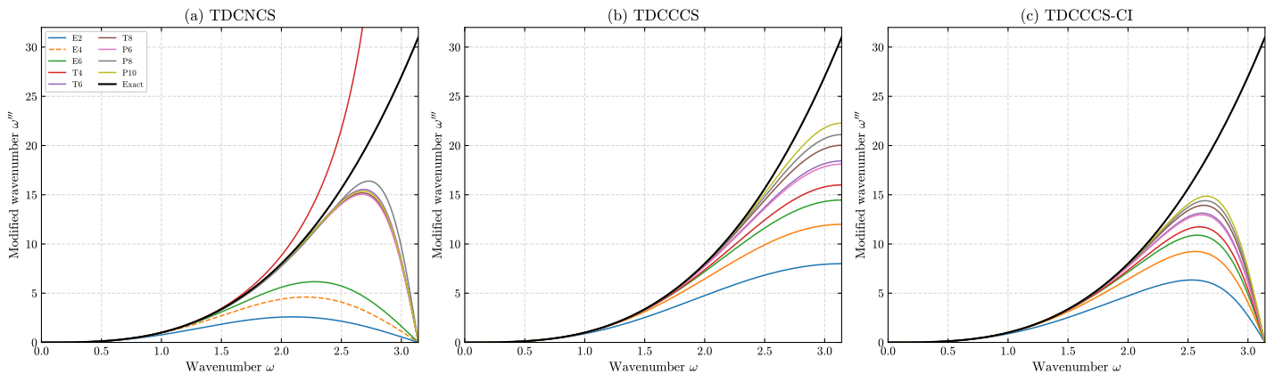
Figure 2: Modified wavenumber against wavenumber for (a) TDCNCS, (b) TDCCCS, and (c) TDCCCS-CI, the last using tenth-order compact interpolation onto the half grid. The T4 curve in panel (a) rises steeply and leaves the plotted range well before $\omega = \pi$; this is a property of the scheme, not an implementation error, since its implicit denominator $1+\cos\omega$ vanishes at $\omega=\pi$.
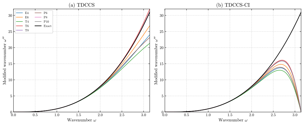
Figure 3: (a) The paper’s new scheme tracks the exact cubic considerably further in wavenumber than TDCNCS or TDCCCS at the same formal order. (b) The degradation incurred by interpolating onto the half grid instead of evolving it directly, which is the transfer error the paper’s design avoids.
The computed bandwidth-resolving efficiencies reproduce the paper’s Tables 5 and 6 to within one unit in the fourth decimal place across every scheme and every operator length:
Table 5 ($\epsilon_t = 10^{-3}$), resolving efficiency $e$:
| Scheme | 4-T computed | 4-T paper | 6-T computed | 6-T paper | 8-T computed | 8-T paper | 10-P computed | 10-P paper |
|---|---|---|---|---|---|---|---|---|
| TDCNCS | 0.2206 | 0.2205 | 0.5523 | 0.5523 | 0.5018 | 0.5018 | 0.5205 | 0.5205 |
| TDCCCS | 0.2278 | 0.2278 | 0.3706 | 0.3705 | 0.4673 | 0.4672 | 0.5874 | 0.5874 |
| TDCCS | 0.2298 | 0.2297 | 0.4412 | 0.4411 | 0.7828 | 0.7828 | 0.9542 | 0.9542 |
Table 6 ($\epsilon_t = 10^{-4}$), resolving efficiency $e$:
| Scheme | 4-T computed | 4-T paper | 6-T computed | 6-T paper | 8-T computed | 8-T paper | 10-P computed | 10-P paper |
|---|---|---|---|---|---|---|---|---|
| TDCNCS | 0.1249 | 0.1248 | 0.4851 | 0.4850 | 0.3856 | 0.3855 | 0.4115 | 0.4114 |
| TDCCCS | 0.1291 | 0.1290 | 0.2545 | 0.2545 | 0.3519 | 0.3518 | 0.4754 | 0.4753 |
| TDCCS | 0.1294 | 0.1294 | 0.2498 | 0.2497 | 0.5376 | 0.5376 | 0.7284 | 0.7284 |
The residual differences of $10^{-4}$ are consistent with the resolution of the wavenumber grid on which $\omega_f$ is located and do not indicate any disagreement in the underlying formulas.
Stability analysis: agreement within grid-resolution noise
The maximum eigenvalue magnitude of each spatial operator was computed directly. For TDCCS this was done by constructing the full $2N\times2N$ coupled operator numerically and calling numpy.linalg.eigvals, without deriving its $2\times2$ Fourier symbol by hand. The result was then combined with the TVDRK3 stability polynomial $R(z) = 1+z+z^2/2+z^3/6$.
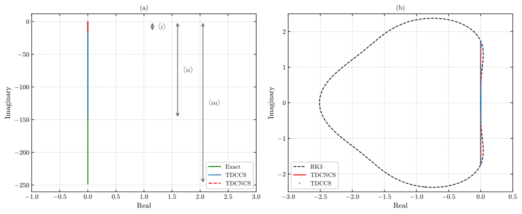
Figure 4: (a) Scaled eigenvalues of the exact, TDCCS and TDCNCS operators over $\omega = k\Delta x \in [0, 2\pi]$. All three are purely imaginary, as a central scheme requires, so each collapses onto the line $\mathrm{Re} = 0$ and the panel reads as three segments of differing length: the exact operator reaches $-(2\pi)^3 \approx -248$, TDCCS $-147.3$, and TDCNCS $-15.2$. The bracketed arrows mark those extents. (b) The TVDRK3 stability region with each operator’s eigenvalues scaled by its own maximum stable CFL number, so that both just reach the imaginary-axis intercept at $\pm1.7321$.
| Quantity | Computed | Paper’s value |
|---|---|---|
| max |eigenvalue|, TDCNCS-T8 | 15.186 | 15.157 |
| max |eigenvalue|, TDCCS-T8 | 147.275 | 147.168 |
| TVDRK3 imaginary-axis intercept | 1.7321 | 1.732 |
| CFL bound $\Delta t/\Delta x^3$, TDCNCS | 0.114 | 0.11 |
| CFL bound $\Delta t/\Delta x^3$, TDCCS | 0.0118 | 0.011 |
5. The six numerical examples
The paper’s Section 7 presents six numerical experiments. Each is stated below in full: the governing equation, the domain and boundary conditions, the initial condition, and the exact solution where one exists. Equation, figure and table numbers follow the paper’s numbering throughout. Every case uses periodic boundary conditions and the TVDRK3 time integrator of Eq. (6.2), with the time step set by Eq. (7.1).
| The error norms follow the paper’s stated definitions, $L^1 = \frac{1}{N+1}\sum_i | u_e - u_a | $ and $L^2 = \big(\frac{1}{N+1}\sum_i | u_e - u_a | ^2\big)^{1/2}$. The tables below show $L^\infty$ only; the reproduction’s $L^1$ values differ from the paper’s by a constant factor, for the reason given in the notes at the end of this post. All 138 convergence rates printed in the paper’s Tables 8 to 11 were also recomputed from the paper’s own printed errors, and every one is consistent with them to within $0.002$. |
Three of the six examples admit closed-form solutions, which permits quantitative error measurement. The remaining three do not, and for those the comparison rests on reproducing the structures the paper describes.
| Example | Governing equation | Exact solution | Figures | Tables |
|---|---|---|---|---|
| 7.1 | Eq. (7.3), linear KdV | yes | 5, 6 | 8, 9 |
| 7.2 | Eq. (7.4), classical soliton | yes | 7 | 10 |
| 7.3 | Eq. (7.5), small dispersion, three sub-cases | single soliton only | 8, 9, 10 | none |
| 7.4 | Eq. (7.5), zero-dispersion limit | no | 11, 12 | none |
| 7.5 | Eq. (7.11), 2D linear dispersion | yes | 13 | 11 |
| 7.6 | Eq. (7.12), Ito-type coupled system | no | 14, 15 | none |
Example 7.1, linear KdV in one dimension
Problem, Eq. (7.3).
\[u_t + c^{-2} u_{xxx} = 0, \qquad (x,t) \in [0, 2\pi] \times [0,1],\]with periodic boundary conditions and the initial condition
\[u(x,0) = \sin(cx), \qquad x \in [0, 2\pi].\]Exact solution. A left-moving wave that retains its shape exactly,
\[u(x,t) = \sin\big(c(x+t)\big).\]Parameters. Two wavenumbers are examined at $N=40$: a low one, $c=1$, giving $k\Delta x = 0.157$, and a higher one, $c=8$, giving $k\Delta x = 1.2566$.
This example contains no convective term, so it exercises only the third-derivative operators the paper defines and tabulates itself. Nothing is borrowed from another source, which makes it the cleanest of the six to reproduce.
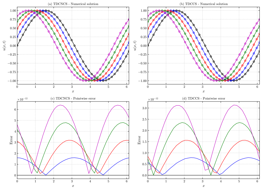
Figure 5: Low-wavenumber case ($c=1$, $N=40$). Top: numerical solution (markers) against the exact traveling wave (lines) at five times. Bottom: pointwise error, on a scale of $10^{-12}$, which is close to the round-off limit of a third-derivative approximation on this grid (Section 3), though still well above machine precision. TDCCS (right) is approximately twice as accurate as TDCNCS (left) at this resolution, in agreement with the paper’s comparison.
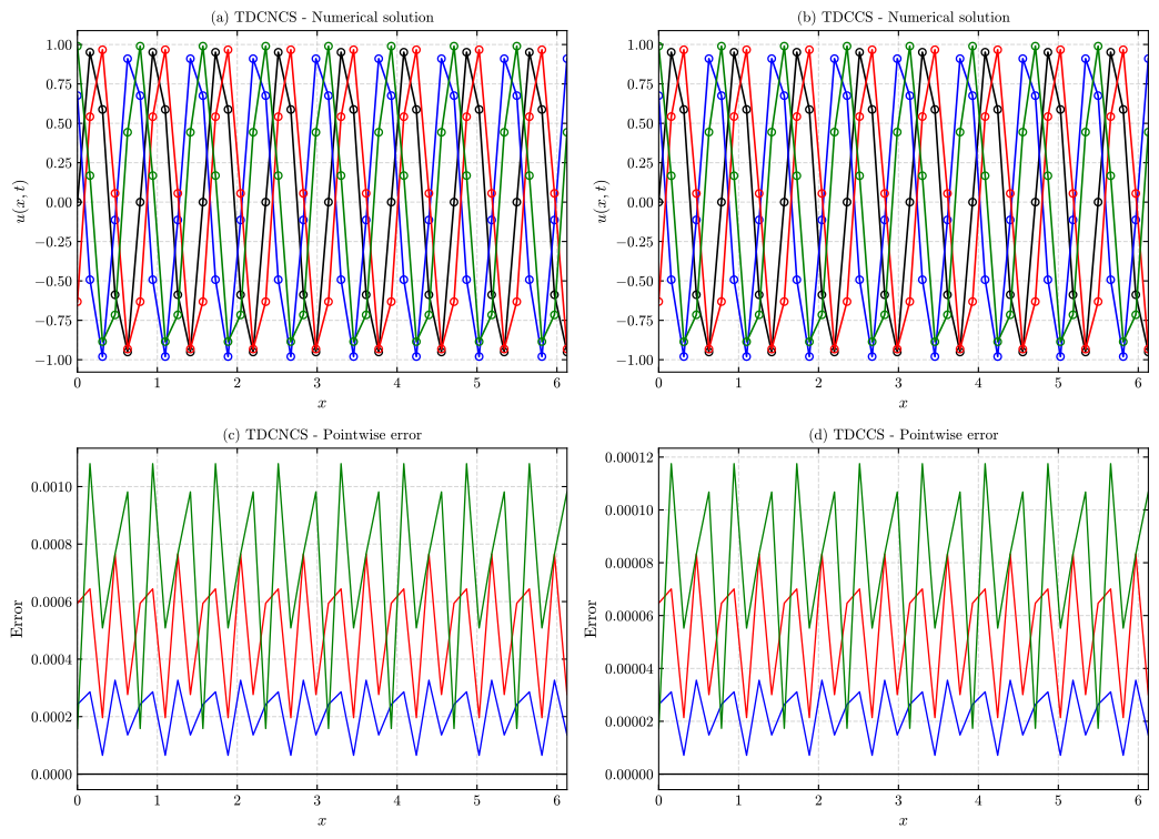
Figure 6: Higher-wavenumber case ($c=8$, $N=40$). The error scale is now $10^{-3}$ to $10^{-4}$, since the grid barely resolves this wavenumber. The superior resolving power of TDCCS evident in Figure 3 appears here directly as an error roughly ten times smaller.
Table 8 ($c=1$), $L^\infty$ error at $t=1$, with convergence rate in parentheses:
| $N$ | TDCNCS (computed) | TDCNCS (paper) | TDCCS (computed) | TDCCS (paper) |
|---|---|---|---|---|
| 10 | 4.1920e-07 | 4.1920e-07 | 1.1729e-07 | 1.1729e-07 |
| 20 | 1.6088e-09 (8.0255) | 1.6089e-09 (8.0254) | 6.4031e-10 (7.5170) | 6.4028e-10 (7.5172) |
| 30 | 6.2206e-11 (8.0224) | 6.2438e-11 (8.0133) | 2.6788e-11 (7.8280) | 2.6557e-11 (7.8493) |
| 40 | 6.4105e-12 (7.8994) | 6.6573e-12 (7.7810) | 3.1374e-12 (7.4547) | 2.9112e-12 (7.6846) |
Agreement is to four or five significant figures at $N=10$ and $N=20$. At $N=30$ and $N=40$ the errors approach the round-off-limited regime of $10^{-11}$ to $10^{-12}$ identified in Section 3, and the computed and published values differ by 0.4 to 8 percent. The rates remain close to eight for both schemes and agree with the paper’s to within about 0.1 to 0.2 at the finest grids. The paper’s rates are correct; an earlier discrepancy in this table was a bug in this reproduction, which computed the rates with $\log_2$ although $N = 10, 20, 30, 40$ does not double. The paper notes that beyond $N=40$ the error stagnates at machine precision.
Table 9 ($c=8$), $L^\infty$ error at $t=1$ (observed rates in parentheses):
| $N$ | TDCNCS (computed) | TDCNCS (paper) | TDCCS (computed) | TDCCS (paper) |
|---|---|---|---|---|
| 20 | 7.9125e-01 | 7.9090e-01 | 8.9768e-03 | 9.4000e-03 |
| 40 | 1.0796e-03 (9.518) | 1.1000e-03 (9.490) | 1.1749e-04 (6.256) | 1.1796e-04 (6.316) |
| 60 | 3.6487e-05 (8.354) | 3.6490e-05 (8.400) | 7.5798e-06 (6.760) | 7.5773e-06 (6.771) |
| 80 | 3.4196e-06 (8.229) | 3.4187e-06 (8.231) | 9.5506e-07 (7.201) | 9.5592e-07 (7.196) |
| 100 | 5.6760e-07 (8.048) | 5.6757e-07 (8.047) | 1.8588e-07 (7.335) | 1.8591e-07 (7.338) |
| 120 | 1.3032e-07 (8.071) | 1.3032e-07 (8.070) | 4.6901e-08 (7.553) | 4.6895e-08 (7.555) |
| 140 | 3.7705e-08 (8.045) | 3.7705e-08 (8.045) | 1.4412e-08 (7.655) | 1.4411e-08 (7.654) |
| 160 | 1.2768e-08 (8.109) | 1.2758e-08 (8.115) | 5.0752e-09 (7.816) | 5.0733e-09 (7.818) |
This is the more informative of the two cases, because at $c=8$ the grid is stressed: $N=40$ gives roughly five points per wavelength. The reproduction covers the paper’s full range, $N=20$ to $160$, which at $N=160$ takes about $1.6\times10^6$ RK3 steps because the time step scales as $\Delta x^3$ (the independent solves were run in parallel, table9_parallel.py). Agreement is to four significant figures from $N=60$ onward and to three at the coarser grids, and the observed rates match the paper’s to within $0.06$ everywhere; at $N=160$ they are $8.109$ against $8.115$ for TDCNCS and $7.816$ against $7.818$ for TDCCS. TDCCS approaches its asymptotic eighth-order rate from below, as the operator test of Section 3 also shows.
The ratio of the two schemes’ errors reproduces the paper’s comparison, with one qualification. TDCCS is more accurate at every resolution, by a factor of $88$ at $N=20$ and $9.2$ at $N=40$, but the factor falls to $3.6$ at $N=80$ and $2.5$ at $N=160$, because TDCNCS converges at the faster rate. The paper’s summary that TDCCS “consistently yields an order of magnitude lower absolute error” holds at the coarse grids, where the grid resolves the wave poorly, and overstates the gain at the fine ones.
Example 7.2, the classical KdV soliton
Problem, Eq. (7.4).
\[u_t - 3(u^2)_x + u_{xxx} = 0, \qquad x \in [-10, 12], \quad t \ge 0,\]with periodic boundary conditions and
\[u(x,0) = -2\,\mathrm{sech}^2(x).\]Exact solution. For $t \in [0, 0.5]$,
\[u(x,t) = -2\,\mathrm{sech}^2(x - 4t),\]the initial profile translated to the right at constant speed $4$, with amplitude and width unchanged.
Parameters. $N=80$ for the figure; $N = 20$ to $160$ for the convergence table, evaluated at $t=0.5$.
The soliton is the standard benchmark for a dispersive solver precisely because its shape is preserved. Nonlinear steepening, which would sharpen the front into a shock, and dispersion, which would spread the pulse into a wave train, cancel exactly. A scheme that mistreats either term distorts the profile visibly, and the distortion accumulates as the wave propagates.
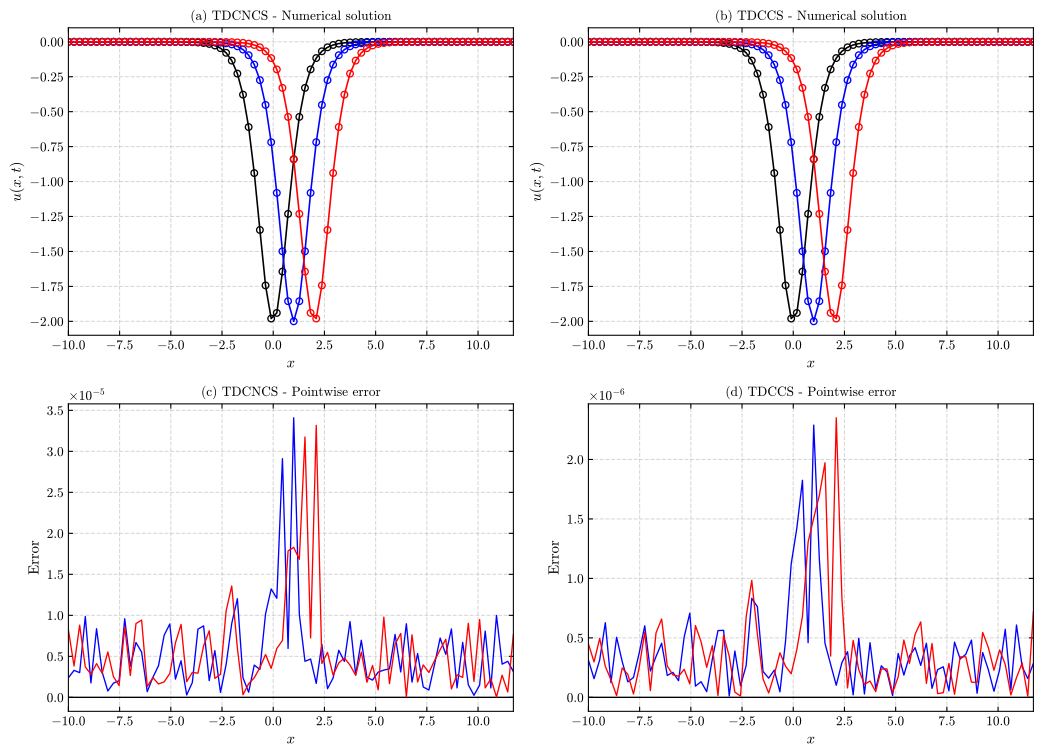
Figure 7: Numerical solution and pointwise error at $t = 0$, $0.25$ and $0.5$ for $u_t - 3(u^2)_x + u_{xxx}=0$, with exact solution $u(x,t)=-2\,\mathrm{sech}^2(x-4t)$, at $N=80$. Panels (a) and (b) show the two schemes against the exact travelling wave; panels (c) and (d) the corresponding errors. The error axes are scaled independently: TDCNCS peaks near $3.5\times10^{-5}$ and TDCCS near $2.4\times10^{-6}$, against the paper’s $3.5\times10^{-5}$ and $2.5\times10^{-6}$.
Table 10, $L^\infty$ error at $t=0.5$, with measured convergence rate:
| $N$ | TDCNCS (computed) | TDCNCS (paper) | Rate | TDCCS (computed) | TDCCS (paper) | Rate |
|---|---|---|---|---|---|---|
| 20 | 5.4859e-01 | 5.4860e-01 | 2.0464e-02 | 2.0500e-02 | ||
| 40 | 1.2990e-02 | 1.3000e-02 | 5.400 | 2.6299e-04 | 2.6299e-04 | 6.282 |
| 60 | 3.2815e-04 | 3.2815e-04 | 9.072 | 1.7387e-05 | 1.7387e-05 | 6.700 |
| 80 | 3.3170e-05 | 3.3170e-05 | 7.967 | 2.3502e-06 | 2.3505e-06 | 6.956 |
| 100 | 5.6879e-06 | 5.6879e-06 | 7.902 | 4.8845e-07 | 4.8863e-07 | 7.040 |
| 120 | 1.3255e-06 | 1.3255e-06 | 7.989 | 1.3146e-07 | 1.3224e-07 | 7.199 |
| 140 | 3.7699e-07 | 3.7699e-07 | 8.157 | 4.2077e-08 | 4.2387e-08 | 7.390 |
| 160 | 1.2705e-07 | 1.2705e-07 | 8.146 | 1.6954e-08 | 1.7577e-08 | 6.807 |
This is the closest agreement obtained anywhere in the reproduction. Six of the eight TDCNCS rows match the published value in every digit reported, and the remaining two differ only in the fifth significant figure. The TDCCS column agrees in every digit at $N=40$ and $N=60$ and to four significant figures at $N=80$ and $N=100$; the differences are 0.2 percent at $N=20$ and grow from 0.6 to 3.5 percent between $N=120$ and $N=160$.
The measured rates reproduce a subtler feature of the paper as well. TDCNCS holds close to its theoretical eighth order across the sweep, settling near $8.0$ to $8.2$, whereas TDCCS stabilizes nearer seven, between $6.8$ and $7.4$ from $N=80$ onward. The paper records the same asymmetry, observing that TDCCS approaches seventh-order accuracy for larger $N$ while TDCNCS maintains a rate close to the theoretical eighth order. Recovering an unexpected and unexplained feature of the original, in addition to its headline numbers, is stronger evidence of a faithful implementation than matching the errors alone would be.
The two schemes are therefore not equivalent in practice. Despite converging at a lower rate, TDCCS is more accurate than TDCNCS at every grid size tested, by a factor between about $7.5$ (at $N=160$) and $49$ (at $N=40$). The paper’s own reading is that TDCCS delivers higher accuracy while TDCNCS remains more efficient per unit of computational cost, since the coupled node-and-center solve roughly doubles the work per step.
Example 7.3, nonlinear KdV with a small dispersion coefficient
Problem, Eq. (7.5).
\[u_t + \left(\frac{u^2}{2}\right)_x + \epsilon\, u_{xxx} = 0,\]with periodic boundary conditions. Three sub-cases follow, corresponding to Sections 7.1, 7.2 and 7.3 of the paper.
With $\epsilon$ of order $10^{-4}$ the dispersive term barely restrains the nonlinear steepening, so the structures that form are narrow and tall. Resolving them demands short-wavelength accuracy, which is the property the Fourier analysis of Figures 2 and 3 quantifies. This example is therefore where that analysis meets a computation.
Single soliton propagation
Initial condition, Eq. (7.6).
\[u(x,0) = 3c\,\mathrm{sech}^2\big(k(x - x_0)\big), \qquad x \in [0,2],\]with $k = \tfrac{1}{2}\sqrt{c/\epsilon}$, $c = 0.3$, $x_0 = 0.5$ and $\epsilon = 5\times10^{-4}$, giving $k \approx 12.25$.
Exact solution. A solitary wave travelling right at speed $c$,
\[u(x,t) = 3c\,\mathrm{sech}^2\Big(k\big[(x - x_0) - ct\big]\Big).\]Parameters. $N=80$, shown at $t = 0, 1, 2, 3$.
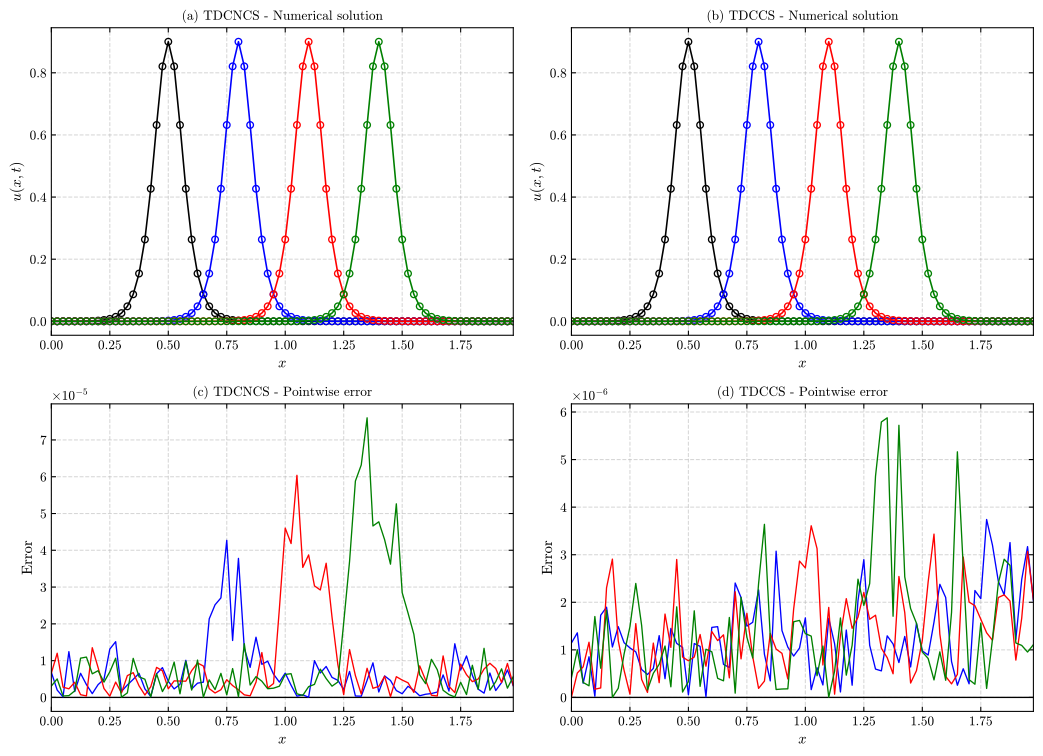
Figure 8: Single soliton propagation at $\epsilon=5\times10^{-4}$, $N=80$, at $t=0$, $1$, $2$ and $3$, matching the paper’s Section 7.1 exactly. TDCNCS (left) uses Lele’s node-only convective scheme; TDCCS (right) uses Liu et al.’s node-and-center scheme, evolved alongside the TDCCS dispersive scheme, consistent with the paper’s stated pairing. With $k = 0.5\sqrt{c/\epsilon} \approx 12.2$ the soliton is a narrow spike, so this tests short-wavelength resolution as much as formal order, and the TDCCS error is smaller by roughly an order of magnitude, as the paper reports.
Double soliton collision
Initial condition, Eq. (7.7). Two solitons superposed,
\[u(x,0) = 3c_1\,\mathrm{sech}^2\big(k_1(x - x_1)\big) + 3c_2\,\mathrm{sech}^2\big(k_2(x - x_2)\big), \qquad x \in [0,2],\]with $k_j = \tfrac{1}{2}\sqrt{c_j/\epsilon}$, $c_1 = 0.3$, $c_2 = 0.1$, $x_1 = 0.4$, $x_2 = 0.8$ and $\epsilon = 4.84\times10^{-4}$.
Exact solution. None available. Taller KdV solitons travel faster, so the leading soliton is overtaken; the diagnostic is whether both emerge from the interaction with their original amplitudes.
Parameters. $N=100$, $t \in [0,4]$.
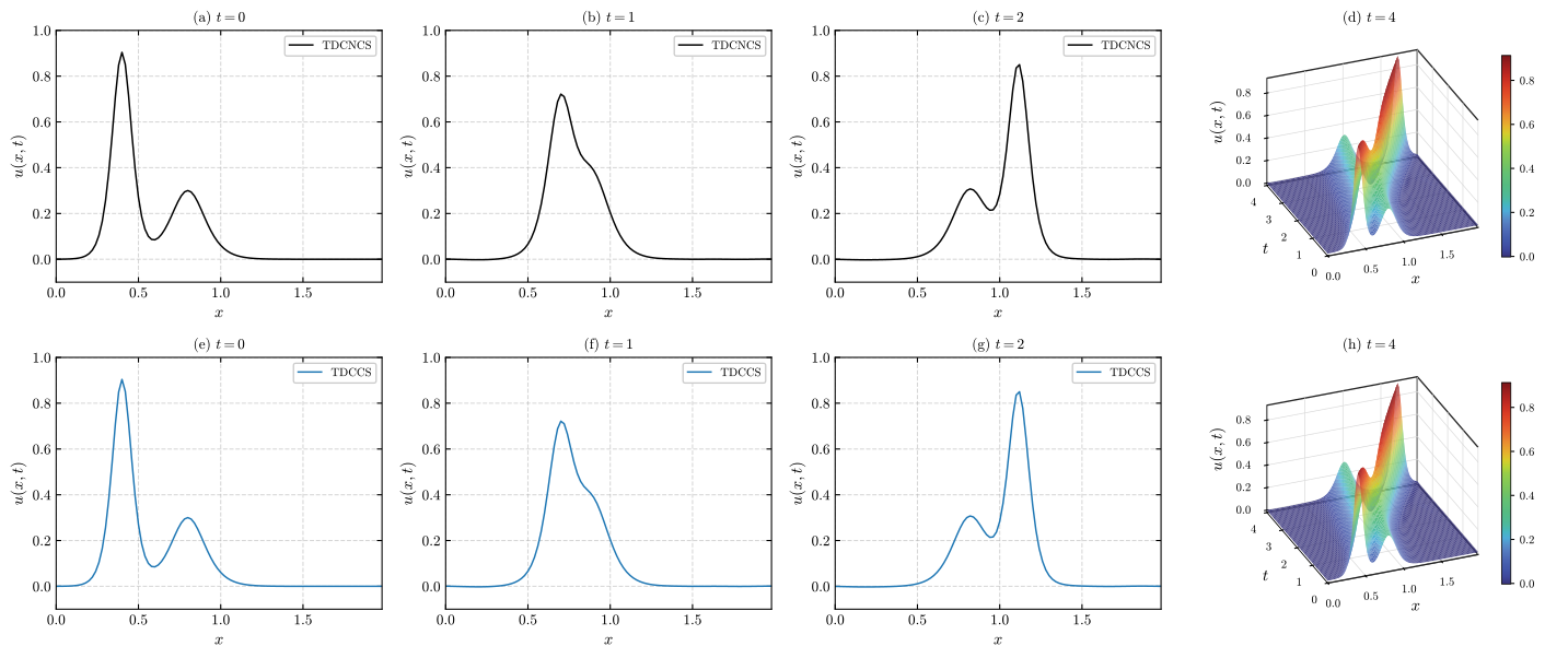
Figure 9: Double soliton collision from the Eq. (7.7) initial condition, at the paper’s parameters ($\epsilon=4.84\times10^{-4}$, $N=100$, $t$ up to $4$). Two rows, TDCNCS above and TDCCS below; the first three columns are snapshots at $t=0$, $1$ and $2$, and the fourth is a space-time surface at $t=4$. The taller soliton, being faster, overtakes the shorter one, and the surfaces show the two ridges meeting and continuing. That both emerge with their original amplitudes is the defining property of solitons, and the paper reports that both schemes handle this case well.
Triple soliton splitting
Initial condition, Eq. (7.8).
\[u(x,0) = \frac{2}{3}\,\mathrm{sech}^2\!\left(\frac{x-1}{\sqrt{108\,\epsilon}}\right), \qquad x \in [0,3],\]with $\epsilon = 10^{-4}$.
Exact solution. None available. This profile is not a soliton, since it does not satisfy the amplitude-width relation a soliton requires, so it cannot propagate unchanged. It breaks into several solitons which then separate, trailed by dispersive ripples.
Parameters. $N=150$, $t$ up to $4$. The twelfth-order filter of Eq. (5.1), with $\alpha_F = 0.4$, is applied every 20 steps for TDCNCS and every 50 steps for TDCCS.
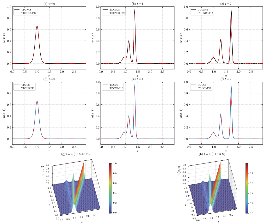
Figure 10: Triple soliton splitting from the Eq. (7.8) initial condition, at the paper’s parameters ($\epsilon=10^{-4}$, $N=150$, $t$ up to $4$). Three rows: TDCNCS at $t=0$, $1$, $2$; then TDCCS at the same times; then two space-time surfaces at $t=4$, one per scheme, computed without the filter. The initial hump is not a soliton, so it cannot travel unchanged; it breaks into several solitons that separate as the taller outrun the shorter, trailed by dispersive ripples. Each line panel overlays the unfiltered run with the same run under the twelfth-order filter (Eq. 5.1, Table 7), applied every 20 steps for TDCNCS and every 50 for TDCCS, as the paper specifies. That asymmetry is itself the paper’s argument: TDCCS resolves short waves better, generates fewer spurious oscillations, and needs less frequent intervention.
Example 7.4, the zero-dispersion limit
Problem. The same nonlinear equation as Example 7.3, Eq. (7.5), examined as $\epsilon \to 0^{+}$.
The paper’s text introduces this example as using “the KdV equation (7.3)”. Eq. (7.3), however, is the linear problem of Example 7.1, which has no convective term and therefore admits no zero-dispersion limit. The equation intended is Eq. (7.5), and that is what is solved here. The captions of Figures 11 and 12 similarly read “Example 7.3”, although the initial conditions they cite, Eqs. (7.9) and (7.10), belong to Example 7.4.
Setting $\epsilon = 0$ exactly reduces the equation to inviscid Burgers, whose solutions form true discontinuities in finite time. For small but non-zero $\epsilon$ the dispersive term forbids a jump, and a packet of rapid oscillations appears in its place. As $\epsilon$ decreases these become faster and more numerous without disappearing, so the solution does not converge pointwise to the shock. The oscillations are physical, not numerical artifacts, which is why the paper observes that low-pass filtering does not affect these results, and why the mesh must be refined as $\epsilon$ falls.
Continuous initial condition, Eq. (7.9).
\[u(x,0) = 2 + \tfrac{1}{2}\sin(2\pi x), \qquad x \in [0,1].\]Discontinuous initial condition, Eq. (7.10).
\[u(x,0) = \begin{cases} 1, & 0.25 < x < 4, \\ 0, & \text{otherwise,} \end{cases} \qquad x \in [0,5].\]Exact solution. None available in either case. For the continuous problem the paper generates a reference solution with TDCNCS on a refined mesh of $N=1000$.
Parameters. Continuous case, evaluated at $t=0.5$: $\epsilon = 10^{-4}$ with $N=100$, $\epsilon = 10^{-5}$ with $N=200$, $\epsilon = 10^{-6}$ with $N=800$, and $\epsilon = 10^{-7}$ with $N=1600$. Top-hat case: $N=1000$ on $x \in [0,5]$, $\epsilon = 10^{-4}$, evaluated at $t=0.01$ and $t=0.05$.
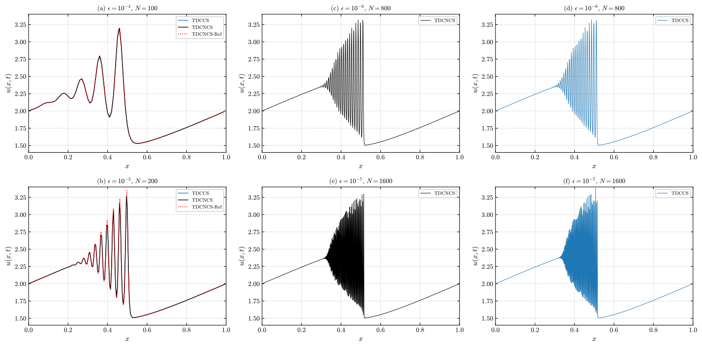
Figure 11: The zero-dispersion limit at $t=0.5$, computed at the paper’s own parameters: $\epsilon$ swept from $10^{-4}$ down to $10^{-7}$ with correspondingly refined grids from $N=100$ to $N=1600$, against a TDCNCS reference at $N=1000$. Panels (a) and (b) place both schemes alongside that reference; panels (c) to (f) show the two finest cases, one scheme per panel, since the oscillations become too dense for overlaid curves to be legible. The rapid oscillations are physical, which is why the paper notes that filtering does not alter these results, and why the mesh must be refined as $\epsilon$ decreases.
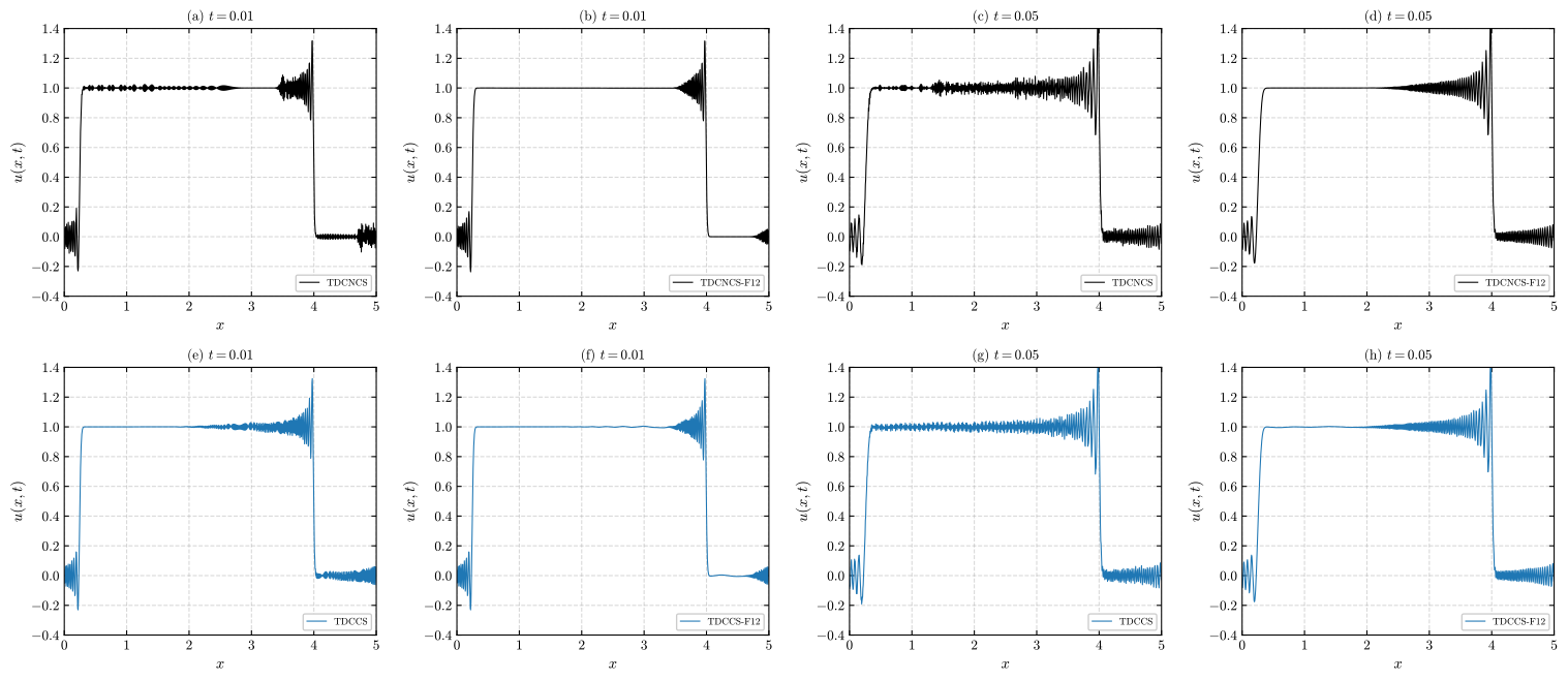
Figure 12: Top-hat breakup at the paper’s parameters ($N=1000$, $\epsilon=10^{-4}$, $x \in [0,5]$). Two rows, TDCNCS above and TDCCS below; within each row the columns run unfiltered and filtered at $t=0.01$, then unfiltered and filtered at $t=0.05$. A discontinuous initial condition contains every wavelength at once, including many the grid cannot represent, so each edge immediately breaks into a train of dispersive waves. Here, unlike in Figure 11, the filter does help: what it removes are grid-scale numerical artifacts, not physical structure, and applying it reduces both the amplitude and the roughness of the train while leaving the propagating packet intact.
Example 7.5, two-dimensional linear dispersion
Problem, Eq. (7.11).
\[u_t + u_{xxx} + u_{yyy} = 0, \qquad (x,y,t) \in (0,2\pi) \times (0,2\pi) \times (0,T],\]with periodic boundary conditions in both directions and
\[u(x,y,0) = \sin(x+y).\]Exact solution.
\[u(x,y,t) = \sin(x + y + 2t).\]Parameters. $N=40$ for the figure, evaluated at $t=1$; $N = 10$ to $40$ in steps of 5 for the convergence table, as in the paper.
Like Example 7.1 this problem has no convective term. For TDCNCS, each third-derivative term is treated by applying the same one-dimensional operator along the corresponding grid direction, so no new construction is required.
TDCCS is a different matter, and the paper does not spell out how its node-and-center pairing extends to two dimensions. In one dimension the state is a pair, values at the nodes and values at the cell centers. On a tensor-product grid each axis carries its own node-center split, so the state becomes four fields instead of two, one for each combination of $(x\text{ node or center}, y\text{ node or center})$. Which fields are paired then matters. Differentiating in $x$ requires node and center values in $x$ taken at the same $y$; differentiating in $y$ requires node and center values in $y$ taken at the same $x$. Pairing fields that sit on different grid lines produces a scheme that remains bounded but loses essentially all accuracy, a failure that presents as poor convergence and not as the indexing error it is.
Two observations support the four-field construction as the one the paper used. First, an initial two-field implementation, pairing values that lay on different $y$ lines, gave an $L^\infty$ error of $1.3\times10^{-1}$ at $N=12$, with no sign of convergence. Second, the four-field version reproduces the paper’s published TDCCS errors exactly at the coarsest grids: $2.4044\times10^{-7}$ at $N=10$ and $1.1687\times10^{-8}$ at $N=15$, matching every digit reported.
A second detail is easy to overlook. Equation (7.2) sets the two-dimensional time step by summing the contributions of both directions, so the admissible step is half what the one-dimensional formula gives on the same grid. Omitting that factor leaves TDCCS unstable here, since Eq. (6.3) already restricts it to $\Delta t/\Delta x^3 \le 0.011$, an order of magnitude tighter than TDCNCS.
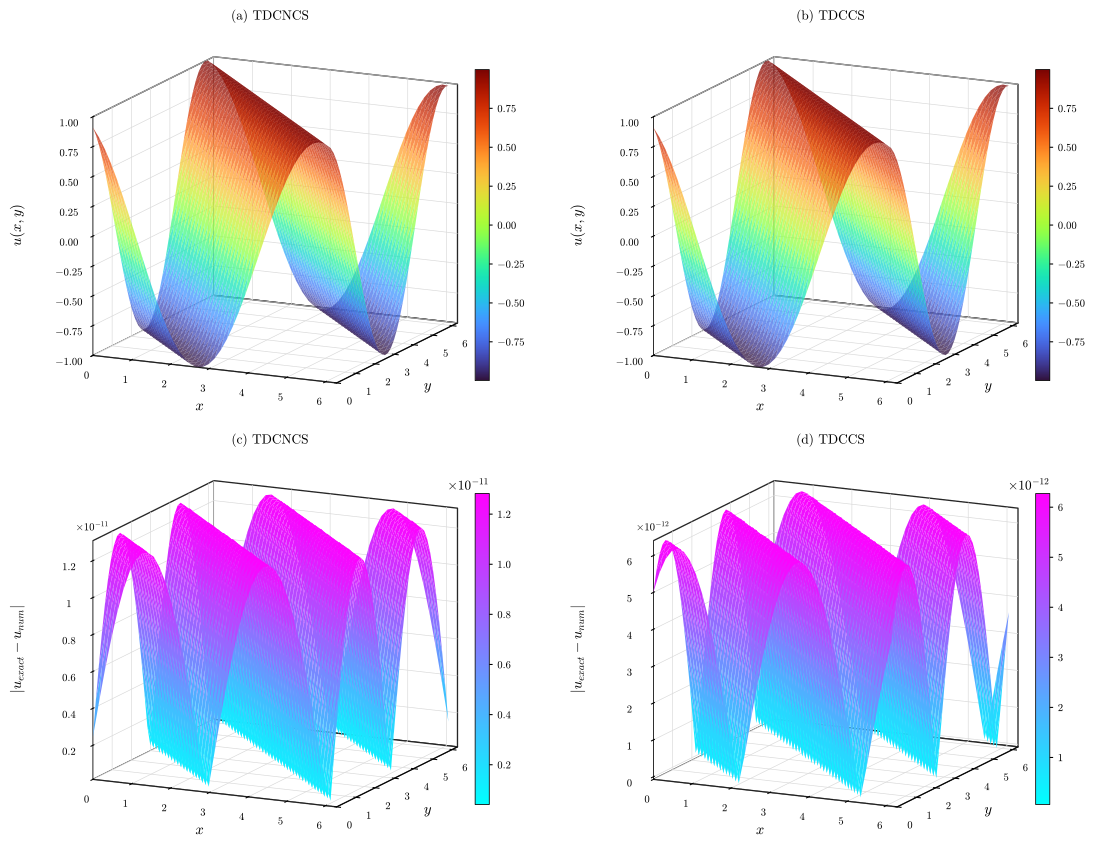
Figure 13: Four surfaces at $t=1$, $N=40$, in the paper’s arrangement. The first column is TDCNCS and the second TDCCS; the top row shows the numerical solution and the bottom row the pointwise error. The diagonal ridges in the error surfaces are not a defect: the exact solution depends on $x$ and $y$ only through $x+y$, so it is constant along lines of constant $x+y$, and the error inherits that structure from the way such a wave meets a square grid.
Table 11, $L^\infty$ error at $t=1$, both schemes (observed rates in parentheses):
| $N$ | TDCNCS (computed) | TDCNCS (paper) | TDCCS (computed) | TDCCS (paper) |
|---|---|---|---|---|
| 10 | 8.6153e-07 | 8.6153e-07 | 2.4044e-07 | 2.4044e-07 |
| 15 | 3.2458e-08 (8.086) | 3.2458e-08 (8.086) | 1.1687e-08 (7.458) | 1.1687e-08 (7.458) |
| 20 | 3.2018e-09 (8.051) | 3.2016e-09 (8.052) | 1.2741e-09 (7.704) | 1.2744e-09 (7.703) |
| 25 | 5.3748e-10 (7.998) | 5.3720e-10 (8.000) | 2.2478e-10 (7.775) | 2.2507e-10 (7.770) |
| 30 | 1.2396e-10 (8.046) | 1.2351e-10 (8.063) | 5.3458e-11 (7.877) | 5.3902e-11 (7.839) |
| 35 | 3.6298e-11 (7.967) | 3.4686e-11 (8.239) | 1.5979e-11 (7.834) | 1.7566e-11 (7.273) |
| 40 | 1.2816e-11 (7.797) | 1.0682e-11 (8.820) | 6.2809e-12 (6.993) | 8.2851e-12 (5.628) |
The reproduction covers the paper’s full range, $N=10$ to $40$. The TDCCS solves at the finest grids are expensive, because the time step scales as $\Delta x^3$ and each step updates four coupled fields on $N^2$ points, so they were run in parallel (table11_parallel.py); $N=40$ took about three hours on a laptop. Both schemes match the published errors in every digit at $N=10$ and $N=15$ and agree to within 0.8 percent through $N=30$, where the rates sit within $0.02$ of the paper’s for TDCNCS and within $0.04$ for TDCCS.
At $N=35$ and $N=40$ the errors reach $10^{-11}$ to $10^{-12}$, the round-off-limited regime of Section 3, and the two sets of numbers separate: the reproduction differs from the paper by 5 to 20 percent for TDCNCS and 9 to 24 percent for TDCCS. The rates show the same thing. The reproduced rates stay close to the scheme’s order (7.97 and 7.80 for TDCNCS, 7.83 and 6.99 for TDCCS), while the paper’s move further from it in both directions (8.24 and 8.82, above the formal order, for TDCNCS; 7.27 and 5.63 for TDCCS). Rates above eight, or falling sharply, in this regime reflect round-off in the particular floating-point operations of each implementation, not the discretization, so neither set of finest-grid rates should be read as a property of the schemes.
Example 7.6, the Ito-type coupled system
Problem, Eq. (7.12).
\[\begin{aligned} u_t - (3u^2 + v^2)_x - u_{xxx} &= 0, \\ v_t - 2(uv)_x &= 0, \end{aligned}\]with periodic boundary conditions.
Initial conditions. Two cases are considered. The trigonometric case, Eq. (7.13),
\[u(x,0) = \cos(x), \qquad v(x,0) = \cos(x), \qquad x \in [0, 2\pi],\]and the Gaussian case, Eq. (7.14),
\[u(x,0) = e^{-x^2}, \qquad v(x,0) = e^{-x^2}, \qquad x \in [-15, 15].\]Exact solution. None available. The paper compares its results against those of Xu and Shu for the same system.
Parameters. Trigonometric case: 80 cells, shown at $t = 0, 0.5, 1$. Gaussian case: 160 cells, shown at $t = 0, 1, 2$. No filtering is applied in either.
The structural feature governing the behavior is visible in the equations themselves: only the $u$ equation carries a third derivative. The $v$ equation is pure nonlinear advection, with nothing to oppose steepening, so $v$ develops shock-type fronts while $u$ remains smooth and dispersive.
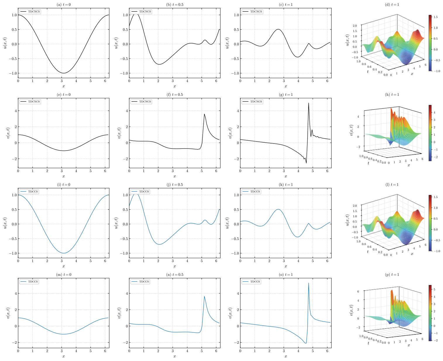
Figure 14: The system $u_t - (3u^2+v^2)_x - u_{xxx}=0$, $v_t - 2(uv)_x=0$ with $u(x,0)=v(x,0)=\cos x$, on $[0,2\pi]$ with 80 cells, in the paper’s four-by-four arrangement. Rows, from the top: TDCNCS $u$, TDCNCS $v$, TDCCS $u$, TDCCS $v$. The first three columns are snapshots at $t=0$, $0.5$ and $1$; the fourth is a space-time surface at $t=1$. Both components start identical yet diverge immediately, for a reason visible in the equations themselves: only the $u$ equation carries a third derivative. With no dispersion to oppose it, nothing prevents $v$ from steepening, and it develops the shock-type profile the paper describes while $u$ stays smooth and dispersive.
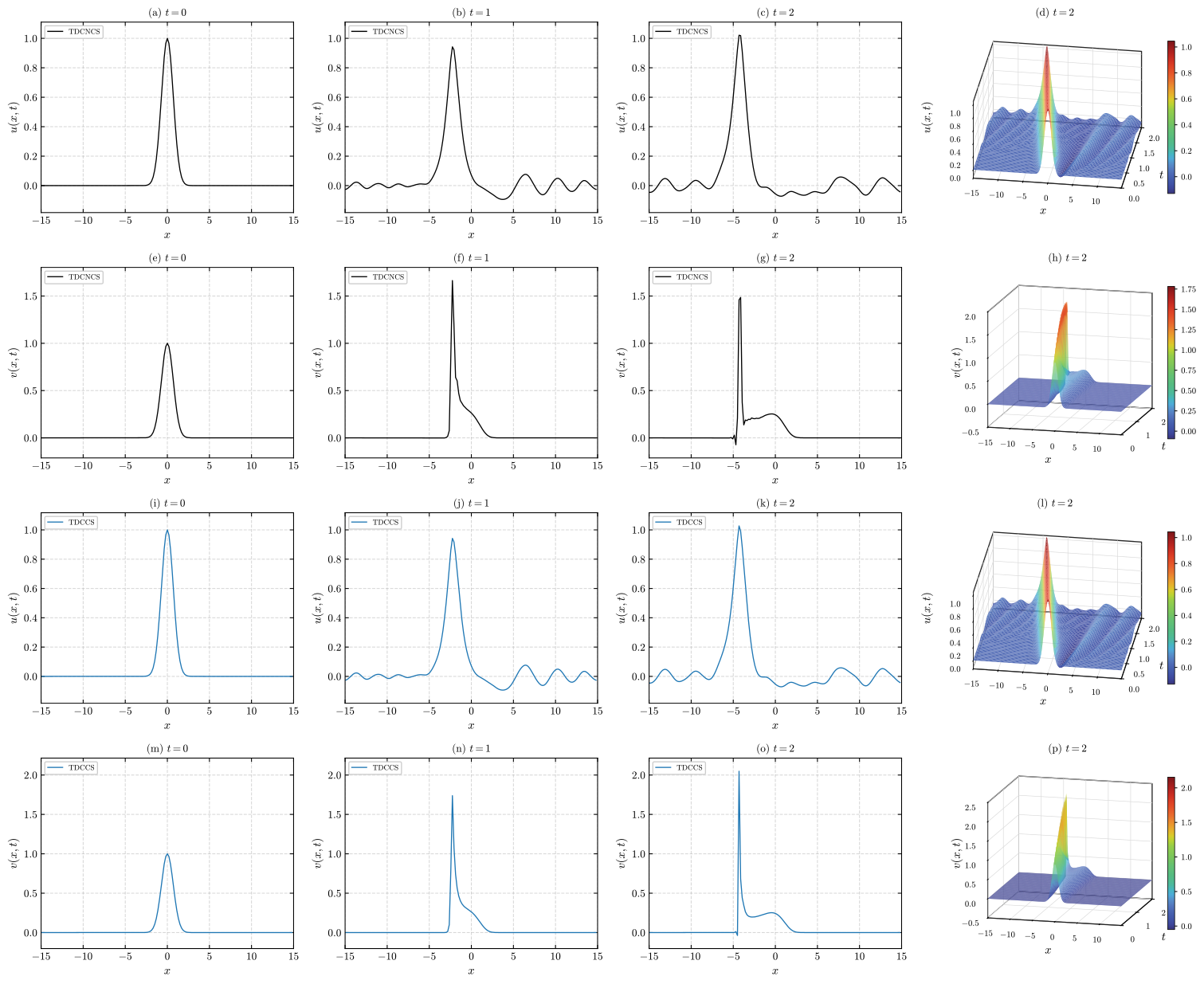
Figure 15: The same system with Gaussian initial data $u(x,0)=v(x,0)=e^{-x^2}$ on $[-15,15]$ with 160 cells, in the same four-by-four arrangement, at $t=0$, $1$ and $2$ with a space-time surface at $t=2$. The wider domain lets the structures separate without wrapping around and interfering with themselves. Both components translate and steepen, and the same asymmetry holds: $v$ forms the steeper front. No filtering is applied in either Ito case, as the paper states explicitly.
6. Reproducing the paper’s figures
The paper’s figures are MATLAB output, and the plots here follow its conventions: axes without padding, surfaces drawn with orthographic projection and without lighting, and the turbo colormap, sampled directly from the paper’s own colorbars where the published figures are stored as CMYK images. The camera angle of each surface panel was measured from the published panel itself, by reading the on-screen directions and lengths of the three axes and solving the orthographic projection equations for elevation and azimuth. All of these conventions, including the camera table, live in pub_style.py, so that no individual figure script sets them independently; the one deliberate departure is that panel labels sit above each axis, which reads better on a web page.
7. Code
The complete code is on GitHub: abelokoj.github.io/_projects/tdccs_project. It is self-contained Python, requiring numpy, scipy, sympy, and matplotlib, and the example scripts are written to be read as a tutorial, each opening with an explanation of the physical problem and how it maps onto the solver.
Computation and plotting are separate. The example scripts solve once and save their results to data/, and a single plotting script, make_figures.py, redraws every surface and snapshot figure from those files. The reason is cost: the stable time step scales like $\Delta x^3$, so the finest runs need hundreds of thousands of Runge-Kutta steps, and recomputing a solution merely to adjust a colour or a camera angle would waste hours. The saved data are included in the repository, so every figure can be redrawn without re-running any solve.
-
tdccs_lib.py: coefficient tables (Tables 1, 2, 3, 4, and 7), modified-wavenumber closures, the periodic circulant solvers for all three third-derivative operators, the first-derivative operators of Lele and of Liu et al., the twelfth-order filter, and TVDRK3. -
nonlinear_kdv.py: the shared nonlinear solvers used by Examples 7.2, 7.3, 7.4 and 7.6. -
derive_order_conditions.py: symbolic Taylor-series derivation of the order conditions for all three schemes. -
verify_tables.py: verification of every published coefficient row against the derived order conditions, and extraction of the leading truncation-error constants. -
validate_operators.py: the grid-refinement tests of the third-derivative operators in Section 3. -
fig_fourier_analysis.py: Figures 2 and 3, Tables 5, 6, and 7. -
fig_stability.py: Figure 4 and the Eq. (6.3) CFL bounds. -
example_7_1_linear_kdv.py: Example 7.1, Tables 8 and 9 and the data for Figures 5 and 6.table9_parallel.pyruns the Table 9 sweep to $N=160$ in parallel. -
example_7_2_soliton.py: Example 7.2, Table 10 and the data for Figure 7. -
example_7_3_solitons.py: Example 7.3, the data for Figures 8, 9 and 10. -
example_7_4_zero_dispersion.py: Example 7.4, the data for Figures 11 and 12. -
example_7_5_2d_linear.py: Example 7.5, Table 11 and the data for Figure 13 (table11_parallel.pyruns the expensive TDCCS rows in parallel). -
example_7_6_ito_system.py: Example 7.6, the data for Figures 14 and 15. -
make_figures.py: draws Figures 5 to 15 from the saved data (python make_figures.py, orpython make_figures.py figure13for one figure). -
figdata.py: saving and loading of the per-figure.npzdata files. -
pub_style.py: the shared publication-qualitymatplotlibstyle (Computer Modern fonts, 600 dpi, PNG, PDF and SVG output) and the MATLAB conventions described in Section 6.
8. Summary of reproduction status
| Result | Status |
|---|---|
| Order-condition derivation (Tables 1, 2, 4) | Exact, verified symbolically: 25 of 26 published rows satisfy every condition they claim. Printed Table 1 (TDCNCS-P8) has the sign of $\beta$ reversed, and printed Eqs. (3.5) to (3.7) are the TDCCCS conditions |
| Truncation-error constants | Exact agreement to all published digits: $3.121917\times10^{-5}$, $6.572523\times10^{-5}$, $-2.188201\times10^{-6}$ |
| Figures 2, 3 (modified wavenumber) | Exact |
| Tables 5, 6 (resolving efficiency) | Agreement to within $10^{-4}$ across all four operator lengths and all three schemes |
| Figure 4, Eq. (6.3) (stability and CFL) | Agreement to three or four significant figures |
| Tables 8, 9, Figures 5, 6 (Example 7.1) | Table 9 ($c=8$) over the paper’s full $N=20$ to $160$: four significant figures from $N=60$, rates within $0.06$. Table 8 ($c=1$): four or five figures at $N=10, 20$, within 0.4 to 8 percent at $N=30, 40$ where the error reaches the $10^{-11}$ to $10^{-12}$ round-off regime, rates within about 0.2 |
| Table 10, Figure 7 (Example 7.2) | Six of eight TDCNCS rows match in every published digit; the rate asymmetry between the schemes is reproduced as well |
| Figures 8, 9, 10 (Example 7.3) | Run at the paper’s grid sizes and integration windows, with the cited convective operators and stated filter intervals |
| Figures 11, 12 (Example 7.4) | Run at the paper’s full $\epsilon$ sweep to $10^{-7}$ and grids to $N=1600$; the oscillatory regime is reached |
| Table 11, Figure 13 (Example 7.5) | Full range $N=10$ to $40$. Both schemes match the published errors in every digit at $N=10$ and $15$ once the four-field two-dimensional pairing is used, and agree to within 0.8 percent through $N=30$; at $N=35, 40$ both are in the round-off regime and differ by 5 to 24 percent |
| Figures 14, 15 (Example 7.6) | Run at the paper’s parameters; the smooth-$u$ against steepening-$v$ asymmetry is reproduced |
Every figure and table in the paper’s Section 7 is reproduced at the paper’s own parameters and over the paper’s full grid ranges, using the first-derivative operators it cites and drawn in the paper’s own panel arrangements.
Where an exact solution exists the agreement is quantitative. Example 7.2 matches the published errors in nearly every reported digit, the two-dimensional results of Example 7.5 match exactly at the coarsest grids, and Examples 7.1 and 7.5 agree to three or four significant figures wherever the error stays above the round-off floor. Where no exact solution exists, in Examples 7.3, 7.4 and 7.6, the comparison is necessarily qualitative and rests on the structures the paper describes: soliton collisions that preserve amplitude, oscillation trains in the zero-dispersion limit, the differing filter intervals the two schemes require, and the smooth-$u$ against steepening-$v$ asymmetry of the Ito system. All are present.
One limitation remains worth stating. The residual differences in the fourth or fifth significant figure at the finest grids of Table 10, and the larger differences at $N \ge 30$ in Table 8, have not been traced individually. They are consistent with round-off accumulating over the very large step counts those runs require, and with the round-off amplification of third-derivative operators shown in Section 3, but that has not been demonstrated.
Notes for readers of the paper
The paper is careful and its numerical conclusions stand; the coefficient tables, truncation-error constants and quantitative examples all reproduce closely. The following small errata may nonetheless help anyone working from it directly:
- Eqs. (3.5) to (3.7). The printed right-hand sides are the TDCCCS (Eq. 2.5) order conditions; the TDCCS conditions derived from Eq. (3.1) are given in Section 2. Table 4 satisfies the derived conditions exactly, so no results are affected.
- Table 1, TDCNCS-P8. The four order conditions determine the row uniquely and give $\beta = +1/166$; the table prints $-1/166$. All other values match, and the row is not used in Section 7.
- $L^1$ norm in Tables 8 to 10. The printed $L^1$ values correspond to dividing by $N$, while the $L^2$ values follow the stated $1/(N+1)$: the reproduction’s $L^1$ differs from the paper’s by exactly $(N+1)/N$ in all 40 rows of Tables 8 to 10, while $L^\infty$ and $L^2$ agree to four digits. Table 11 is consistent, and the effect on the rates is negligible. The reproduction follows the stated definition, which is why its $L^1$ column differs.
- Example 7.5 text. The TDCNCS error at $N=40$ is quoted as $1.0682\times10^{-12}$; Table 11 gives $1.0682\times10^{-11}$.
- “Machine precision.” The error floors near $10^{-12}$ in Examples 7.1, 7.2 and 7.5 are attributed to machine precision, but double-precision epsilon is about $2\times10^{-16}$. The floor is round-off amplified by the third-derivative stencil, as the operator test in Section 3 shows: below about $10^{-11}$ the error grows with $N$ instead of falling.
- Captions and cross-references. Figures 11 and 12 are labelled Example 7.3 (Example 7.4 intended); Figure 13 and Table 11 are labelled Example 7.6 (Example 7.5 intended); Figures 14 and 15 cite “Example (7.12)” (Example 7.6, whose system is Eq. 7.12); and the text of Example 7.4 refers to “the KdV equation (7.3)” where Eq. (7.5) is meant.
As a positive check, all 138 convergence rates printed in Tables 8 to 11 are consistent with the paper’s own printed errors, and every other number quoted in the text matches its table.
References
The compact finite-difference framework used throughout traces to (Lele, 1992), which also supplies the eighth-order node-only first-derivative operator used for the TDCNCS convective term. The central compact scheme coupling node and cell-center values is due to (Liu et al., 2013), whose CCS-T8 row provides the TDCCS convective operator. The scheme reproduced in this post, together with the numerical examples of its Section 7, is that of (Salian et al., 2026), available as a PDF from the author’s website.
- Lele, S. K. (1992). Compact Finite Difference Schemes With Spectral-Like Resolution. Journal of Computational Physics, 103(1), 16–42.
- Salian, L. V., Samala, R., & Ghosh, D. (2026). Central Compact Finite-Difference Scheme With High Spectral Resolution for KdV Equation. Numerical Methods for Partial Differential Equations, 42(1), e70060. https://doi.org/10.1002/num.70060
- Liu, X., Zhang, S., Zhang, H., & Shu, C.-W. (2013). A New Class of Central Compact Schemes With Spectral-Like Resolution I: Linear Schemes. Journal of Computational Physics, 248, 235–256.
The full code for this post, including the saved data behind every figure, is available on GitHub; the scripts are listed in Section 7.