How the numbers were produced. All four libraries were run in a single process on one train/test split of the same dataset, with every random seed fixed, so the results below are directly comparable. The script that produced them is linked at the end of the post.
Motivation
Machine learning is not a single tool but a spectrum of methods, and one of the more useful things an applied mathematician brings to a machine learning team is judgment about where on that spectrum a given problem lies, instead of applying the same deep architecture whatever the data. This post is organized around that principle: one dataset, one problem and four libraries, so that the comparison is between methods and not between unrelated examples.
The four libraries fall into two families:
- scikit-learn and XGBoost (Pedregosa et al., 2011)(Chen & Guestrin, 2016) represent classical statistical learning: linear models, kernel methods, and ensembles of decision trees. Their training problems are convex or close to it, they are well understood theoretically and fast to fit, and, as the results below show, they are often hard to beat on small and medium-sized tabular data.
- TensorFlow/Keras and PyTorch (Abadi Martı́n et al., 2016)(Chollet & others, 2015)(Paszke et al., 2019) represent deep learning: differentiable function approximators trained by stochastic gradient descent and backpropagation, which pay off on high-dimensional, unstructured data such as images, text and audio, or on very large datasets.
The running example
Every library below solves the same problem: binary classification on the Breast Cancer Wisconsin (Diagnostic) dataset (Wolberg et al., 1995), comprising 569 samples and 30 real-valued features derived from digitized images of fine needle aspirate biopsies, labeled malignant or benign. It suits this comparison because it is small, tabular and well separated, which is exactly the regime in which the reflex to reach for a neural network deserves scrutiny.
\[\mathbf{x} \in \mathbb{R}^{30}, \qquad y \in \{0, 1\} \ (\text{malignant}=0,\ \text{benign}=1).\]Part 1: Classical ML with scikit-learn
The main strength of scikit-learn is less any single algorithm than its consistent interface: every estimator implements fit and predict, every preprocessing step composes into a Pipeline, and cross-validation, metrics and hyperparameter search work the same way whichever model is plugged in. That uniformity reduces a fair four-way comparison to a few dozen lines of code instead of four bespoke training scripts.
from sklearn.datasets import load_breast_cancer
from sklearn.model_selection import train_test_split, StratifiedKFold, cross_validate
from sklearn.preprocessing import StandardScaler
from sklearn.pipeline import Pipeline
from sklearn.linear_model import LogisticRegression
from sklearn.svm import SVC
from sklearn.calibration import CalibratedClassifierCV
from sklearn.ensemble import RandomForestClassifier, GradientBoostingClassifier

data = load_breast_cancer()
X, y = data.data, data.target

X_train, X_test, y_train, y_test = train_test_split(
    X, y, test_size=0.25, stratify=y, random_state=42
)

models = {
    "Logistic Regression": Pipeline([
        ("scale", StandardScaler()),
        ("clf", LogisticRegression(max_iter=5000, random_state=42)),
    ]),
    "SVM (RBF kernel)": Pipeline([
        ("scale", StandardScaler()),
        ("clf", CalibratedClassifierCV(SVC(kernel="rbf", random_state=42),
                                       ensemble=False)),
    ]),
    "Random Forest": Pipeline([
        ("clf", RandomForestClassifier(n_estimators=300, random_state=42)),
    ]),
    "Gradient Boosting": Pipeline([
        ("clf", GradientBoostingClassifier(n_estimators=200, learning_rate=0.05,
                                            max_depth=3, random_state=42)),
    ]),
}
The tree-based models omit the StandardScaler step. A decision tree’s splits are unaffected by monotonic rescaling of a feature, so standardization gains nothing there, whereas it is essential for the SVM and logistic regression, whose objectives are not scale-invariant.
Cross-validated comparison
Stratified 5-fold cross-validation on the training set gives:
5-fold cross-validation on training set:
Logistic Regression    acc=0.9789±0.0088  auc=0.9962  f1=0.9833
SVM (RBF kernel)       acc=0.9718±0.0057  auc=0.9951  f1=0.9776
Random Forest          acc=0.9578±0.0175  auc=0.9880  f1=0.9665
Gradient Boosting      acc=0.9554±0.0227  auc=0.9876  f1=0.9642
And on the held-out test set:
Held-out test set performance:
Logistic Regression    test_acc=0.9860  test_auc=0.9977
SVM (RBF kernel)       test_acc=0.9790  test_auc=0.9969
Random Forest          test_acc=0.9580  test_auc=0.9949
Gradient Boosting      test_acc=0.9580  test_auc=0.9929
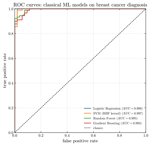
Figure 1: ROC curves on the held-out test set. All four models separate the classes well, with test AUC between 0.993 and 0.998. The best of them is the simplest: logistic regression.
This result deserves attention. The simplest model in the comparison, plain logistic regression, has the best test AUC and the best test accuracy, ahead of both tree ensembles, and it also leads in cross-validation, so it is not an accident of one split. It reflects a property of the data: once the features are standardized, the two classes are close to linearly separable. It also shows that a more flexible model is not automatically a better one, since flexibility the problem does not need adds variance without reducing bias. Formally, for a hypothesis class $\mathcal{H}$ with expected test error decomposed as $\mathbb{E}[(\hat{f}(x) - f(x))^2] = \text{Bias}^2 + \text{Variance} + \sigma^2$, adding capacity beyond what the true decision boundary requires can reduce bias only at the cost of variance; if the boundary is already close to linear, that exchange yields no net benefit.
Where the signal comes from
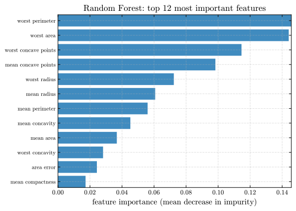
Figure 2: Random Forest feature importances (mean decrease in impurity), top 12 of 30 features. A handful of features, all measures of cell-nucleus size and of the irregularity of its outline, dominate the model’s decisions.
Importance scores of this kind are one of the real advantages tree ensembles keep over deep networks on tabular data: they come almost free as a by-product of training, with no separate post hoc interpretability method.
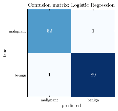
Figure 3: Confusion matrix for logistic regression, the best model by test AUC, on the 143 held-out samples. Two misclassifications in total: one malignant case predicted benign, and one benign case predicted malignant. The errors are symmetric, which the accuracy figure alone does not show, and in a diagnostic setting the two kinds of error are not equally costly.
One implementation detail in the code above is easy to pass over. A support vector machine outputs decision-function values, not probabilities, so drawing its ROC curve requires a calibration step to convert them. The pipeline uses CalibratedClassifierCV(SVC(), ensemble=False), which fits that conversion explicitly. The older route was SVC(probability=True), which performs the same Platt scaling internally; scikit-learn deprecated it in version 1.9 and will remove it in 1.11, and recommends this replacement.
The two yield the same AUC to four decimal places, as expected: AUC depends only on the ranking of the scores, and any monotone recalibration leaves that ranking unchanged. Threshold-dependent metrics do vary slightly, since the two fit their sigmoid on different internal folds, and a few borderline cases cross the $p=0.5$ boundary as a result. Cross-validated accuracy moves from $0.9671$ to $0.9718$ and F1 from $0.9740$ to $0.9776$; test-set accuracy is unchanged at $0.9790$. The distinction between rank-based and threshold-based metrics is worth keeping in mind whenever models with differently calibrated scores are compared.
Part 2: Gradient boosting at scale with XGBoost
The GradientBoostingClassifier of scikit-learn used above is a legitimate gradient boosting implementation (Friedman, 2001), but XGBoost (Chen & Guestrin, 2016), like its relatives LightGBM and CatBoost, improves on it in ways that made gradient-boosted trees the standard choice for tabular prediction. The mathematical difference is worth stating precisely. Where classical gradient boosting fits each new tree to the negative gradient of the loss, a first-order, steepest-descent-style step, XGBoost fits each tree using a second-order Taylor expansion of the loss function around the current prediction,
where $g_i = \partial_{\hat{y}} \ell(y_i, \hat{y}^{(t-1)})$ and $h_i = \partial^2_{\hat{y}} \ell(y_i, \hat{y}^{(t-1)})$ are the first and second derivatives of the loss with respect to the current prediction. The procedure is Newton’s method applied tree by tree, in place of plain gradient descent. The regularization term $\Omega(f_t)$ penalizes tree complexity, specifically the number of leaves as well as the magnitude of leaf weights, directly in the objective, which is a large part of why XGBoost overfits less readily than earlier boosting implementations.
import xgboost as xgb
from sklearn.model_selection import train_test_split, StratifiedKFold, cross_val_score
from sklearn.datasets import load_breast_cancer
from sklearn.metrics import roc_auc_score, accuracy_score

data = load_breast_cancer()
X, y = data.data, data.target
X_train, X_test, y_train, y_test = train_test_split(
    X, y, test_size=0.25, stratify=y, random_state=42
)

model = xgb.XGBClassifier(
    n_estimators=300,
    max_depth=3,
    learning_rate=0.05,
    subsample=0.8,
    colsample_bytree=0.8,
    reg_lambda=1.0,          # L2 regularization on leaf weights
    eval_metric="logloss",
    random_state=42,
)

cv = StratifiedKFold(n_splits=5, shuffle=True, random_state=42)
cv_auc = cross_val_score(model, X_train, y_train, cv=cv, scoring="roc_auc")
print(f"XGBoost CV AUC: {cv_auc.mean():.4f} +/- {cv_auc.std():.4f}")

# No eval_set: the test set is touched once, for the final score only.
model.fit(X_train, y_train, verbose=False)
y_prob = model.predict_proba(X_test)[:, 1]
y_pred = model.predict(X_test)
print(f"Test accuracy: {accuracy_score(y_test, y_pred):.4f}")
print(f"Test ROC-AUC:  {roc_auc_score(y_test, y_prob):.4f}")

# Feature importance, directly comparable to the Random Forest plot above
xgb.plot_importance(model, max_num_features=12, importance_type="gain")
XGBoost CV AUC: 0.9926 +/- 0.0070
Test accuracy: 0.9720
Test ROC-AUC:  0.9950
XGBoost’s test AUC of $0.9950$ is slightly above scikit-learn’s GradientBoostingClassifier ($0.9929$) and level with the Random Forest ($0.9949$; a difference of $10^{-4}$ is noise on 143 test samples). Its test accuracy of $0.9720$ is 1.4 points above both ensembles, which on this test set is two samples. It remains below plain logistic regression ($0.9977$), and its test accuracy of $0.9720$ is likewise below logistic regression’s $0.9860$. The second-order updates and built-in regularization do real work relative to the other tree ensembles, but they cannot change the fact that this dataset is nearly linearly separable.
The top features by gain, shown in Figure 4, are worst radius ($22.09$) and worst perimeter ($22.04$), followed by worst concave points ($14.34$) and mean concave points ($11.77$). These are the same quantities the Random Forest ranked highest: two different ensemble algorithms, with different splitting criteria and different regularization, agree on which measurements carry the diagnostic signal.
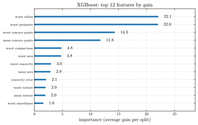
Figure 4: XGBoost feature importances by gain, top 12 of 30, measured as the average improvement in the objective over every split that used the feature. The ordering closely matches the Random Forest ranking in Figure 2. Where the two rankings differ, the difference is informative. XGBoost places worst radius first at $22.09$, where the Random Forest places it fifth, and demotes worst area from second to sixth. Radius, perimeter, and area are close to functionally dependent for a roughly convex shape, so the three carry largely the same information; which of them a given ensemble credits is partly a matter of which happened to be selected first at a split, and the split ordering is not the same under mean-decrease-in-impurity as it is under gain.
On a dataset this small and clean, the differences among the tree ensembles amount to one or two test samples. Each sample is $0.7$ percentage points of test accuracy here, so small gaps should not be read as rankings. Its real advantages (built-in regularization, second-order updates, native handling of missing values and much faster histogram-based split finding) show more decisively on larger, noisier, higher-dimensional tabular data (Shwartz-Ziv & Armon, 2022). With 569 well-separated rows there is simply not enough difficulty for them to matter.
Part 3: Deep learning with TensorFlow/Keras
Deep learning departs from the methods above in its architecture. Instead of choosing a fixed model family (a hyperplane, a kernel expansion, an ensemble of trees) and fitting its parameters, layers are composed into a flexible function approximator whose parameters are found by stochastic gradient descent through backpropagation. Keras (Chollet & others, 2015), the high-level API of TensorFlow (Abadi Martı́n et al., 2016), makes that composition almost declarative:
import tensorflow as tf
from tensorflow import keras
from sklearn.datasets import load_breast_cancer
from sklearn.model_selection import train_test_split
from sklearn.preprocessing import StandardScaler

data = load_breast_cancer()
X, y = data.data, data.target
X_train, X_test, y_train, y_test = train_test_split(
    X, y, test_size=0.25, stratify=y, random_state=42
)

scaler = StandardScaler()
X_train = scaler.fit_transform(X_train)
X_test = scaler.transform(X_test)

model = keras.Sequential([
    keras.layers.Input(shape=(30,)),
    keras.layers.Dense(32, activation="relu"),
    keras.layers.Dropout(0.3),
    keras.layers.Dense(16, activation="relu"),
    keras.layers.Dense(1, activation="sigmoid"),
])

model.compile(
    optimizer=keras.optimizers.Adam(learning_rate=1e-3),
    loss="binary_crossentropy",
    metrics=["accuracy", keras.metrics.AUC(name="auc")],
)

history = model.fit(
    X_train, y_train,
    validation_split=0.2,
    epochs=100,
    batch_size=32,
    callbacks=[keras.callbacks.EarlyStopping(patience=10, restore_best_weights=True)],
    verbose=0,
)

test_loss, test_acc, test_auc = model.evaluate(X_test, y_test, verbose=0)
print(f"Test accuracy: {test_acc:.4f}, Test AUC: {test_auc:.4f}")
epochs actually run: 100 of 100
best val_loss epoch: 95  (weights restored to this)
Test accuracy: 0.9720, Test AUC: 0.9937
trainable params: 1537
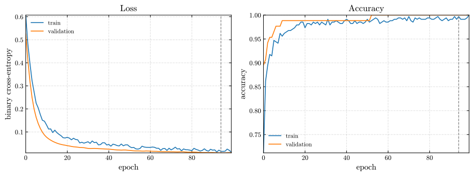
Figure 5: Keras training history. The dashed line marks epoch 95, where validation loss reached its minimum. Both losses fall steeply over the first 20 epochs and then decline slowly for the rest of the run, so early stopping never triggers within the 100-epoch limit. Validation loss sits below training loss throughout, the expected effect of dropout: it is active during training and disabled at evaluation, so the model is scored in a slightly stronger configuration than the one being fitted.
The network has 1,537 trainable parameters, against 426 training samples, roughly 3.6 parameters per example. In this run it used all 100 permitted epochs, with its best validation loss at epoch 95: validation loss was still drifting down, very slowly, so the patience-10 rule never fired. The run is reproducible (seeds fixed, deterministic TensorFlow kernels), but the exact epoch counts depend on the library build; an earlier run under a different TensorFlow installation stopped at epoch 49 with essentially the same test scores. The accuracy is what matters here, and it is stable.
Three points are worth stating precisely:
- The loss. Binary cross-entropy is the negative log-likelihood under a Bernoulli model of the labels, $\mathcal{L} = -\frac{1}{n}\sum_i \left[y_i \log \hat{y}_i + (1-y_i)\log(1-\hat{y}_i)\right]$, which is the same objective that logistic regression minimizes. The network here is, in a precise sense, a nonlinear generalization of the logistic regression model from Part 1, with the sigmoid output layer serving the same role.
- Dropout (Srivastava et al., 2014) (
Dropout(0.3)) randomly zeroes $30\%$ of the hidden units at each training step, preventing the network from depending on any single neuron. It plays a role similar to XGBoost’s leaf-weight penalty, though by a different mechanism: it prevents co-adaptation of units stochastically, where XGBoost adds an explicit norm penalty. - Early stopping halts training once validation loss stops improving, which both regularizes the model and saves compute. It is conceptually similar to limiting
n_estimatorsin tree ensembles, but is set automatically from held-out performance instead of being fixed in advance.
The results make the central comparison concrete. The network reaches a test accuracy of $0.9720$ and a test AUC of $0.9937$, both below logistic regression. All AUCs in this post are computed the same way, with scikit-learn’s exact roc_auc_score; Keras’s built-in metrics.AUC is a 200-bin approximation and reports a slightly different figure. A 1,537-parameter network trained for 100 epochs with dropout has arrived just short of a 31-parameter linear model fitted in a fraction of a second.
This is the point of the exercise. The network is not underperforming because it is misconfigured: the architecture and training procedure are sound, and early stopping shows the regularization working as intended. The dataset is small, tabular and nearly linearly separable, so a linear decision boundary is already very nearly the right hypothesis, and extra capacity has nothing left to fit.
Part 4: The same network in PyTorch
Implementing the identical architecture in PyTorch (Paszke et al., 2019) is instructive, because once syntax is set aside, the differences that remain show when each framework is the better choice.
import torch
import torch.nn as nn
import torch.optim as optim
from torch.utils.data import DataLoader, TensorDataset
from sklearn.datasets import load_breast_cancer
from sklearn.model_selection import train_test_split
from sklearn.preprocessing import StandardScaler
from sklearn.metrics import roc_auc_score

data = load_breast_cancer()
X, y = data.data, data.target
X_train, X_test, y_train, y_test = train_test_split(
    X, y, test_size=0.25, stratify=y, random_state=42
)
scaler = StandardScaler()
X_train = scaler.fit_transform(X_train)
X_test = scaler.transform(X_test)

X_train_t = torch.tensor(X_train, dtype=torch.float32)
y_train_t = torch.tensor(y_train, dtype=torch.float32).unsqueeze(1)
X_test_t = torch.tensor(X_test, dtype=torch.float32)
y_test_t = torch.tensor(y_test, dtype=torch.float32).unsqueeze(1)

class BreastCancerNet(nn.Module):
    def __init__(self):
        super().__init__()
        self.net = nn.Sequential(
            nn.Linear(30, 32),
            nn.ReLU(),
            nn.Dropout(0.3),
            nn.Linear(32, 16),
            nn.ReLU(),
            nn.Linear(16, 1),   # logits -- no sigmoid here, see loss below
        )

    def forward(self, x):
        return self.net(x)

model = BreastCancerNet()
criterion = nn.BCEWithLogitsLoss()   # combines sigmoid + BCE for numerical stability
optimizer = optim.Adam(model.parameters(), lr=1e-3)

n_train = int(0.8 * len(X_train_t))
X_tr, X_val = X_train_t[:n_train], X_train_t[n_train:]
y_tr, y_val = y_train_t[:n_train], y_train_t[n_train:]

# Minibatches of 32, as in the Keras model: roughly 11 optimizer steps per epoch.
loader = DataLoader(TensorDataset(X_tr, y_tr), batch_size=32, shuffle=True)

best_val_loss, patience, patience_ctr = float("inf"), 10, 0
for epoch in range(100):
    model.train()
    for xb, yb in loader:
        optimizer.zero_grad()
        loss = criterion(model(xb), yb)
        loss.backward()
        optimizer.step()

    model.eval()
    with torch.no_grad():
        val_loss = criterion(model(X_val), y_val).item()
    if val_loss < best_val_loss:
        best_val_loss, patience_ctr = val_loss, 0
        best_state = {k: v.clone() for k, v in model.state_dict().items()}
    else:
        patience_ctr += 1
        if patience_ctr >= patience:
            break

model.load_state_dict(best_state)
model.eval()
with torch.no_grad():
    test_prob = torch.sigmoid(model(X_test_t)).numpy().ravel()
test_auc = roc_auc_score(y_test, test_prob)
print(f"Test AUC: {test_auc:.4f}")
The script trains this network twice: once exactly as above, and once with the inner loop replaced by a single full-batch step per epoch (model(X_tr) on the whole training tensor), which is how the loop is often first written.
[full batch] epochs run: 100 of 100, best val_loss epoch: 100, optimizer steps: 100
[full batch] Test accuracy: 0.9510, Test AUC: 0.9943
[minibatch (32)] epochs run: 76 of 100, best val_loss epoch: 66, optimizer steps: 836
[minibatch (32)] Test accuracy: 0.9580, Test AUC: 0.9935
trainable params: 1537
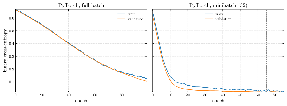
Figure 6: PyTorch training histories. Left, full-batch training: one optimizer step per epoch, and both losses are still falling in a straight line at the 100-epoch limit, with validation loss near $0.10$. Right, minibatches of 32: the loss drops below $0.05$ within about 20 epochs, early stopping fires at epoch 76, and the best validation loss (dashed line, epoch 66) is about $0.02$.
The two runs use the same architecture, loss, optimizer, learning rate and early-stopping rule, and the same 1,537 weights. They differ only in how many optimizer steps each epoch takes: 100 steps in total for the full-batch run against 836 for the minibatch run. The full-batch run never converges. Its best validation loss is at the last epoch, so early stopping never fires, and its test accuracy of $0.9510$ is that of a model interrupted partway through fitting. This is undertraining, not overfitting: an overfitting network has learned the training set too well and must be stopped, while this one had not finished learning.
With minibatches the network converges and reaches $0.9580$ accuracy and $0.9935$ AUC, close to the Keras result, which is what the matching architecture should produce. The trap is worth remembering because the two versions look equivalent on the page. In Keras the step count follows from a batch_size argument; in a hand-written PyTorch loop it follows from what the loop passes to the model, which is easy to overlook. Reproducing a Keras result in PyTorch requires iterating over minibatches, ordinarily through a DataLoader.
The point is not that one framework is more accurate. Both compute the same thing. The explicitness that is PyTorch’s main advantage carries an obligation: decisions a higher-level API makes for the user become the user’s own, including ones the user may not notice making.
Beyond syntax, three structural differences stand out:
- Explicit training loop. The
nn.Moduleof PyTorch provides aforwardmethod and requires the epoch loop, gradient zeroing, backward pass, and optimizer step to be written explicitly, whereasmodel.fitin Keras encapsulates all of this in a single call. The extra code is a trade-off, not just verbosity: the explicitness of PyTorch makes it considerably easier to implement custom training logic, such as multiple losses, custom gradient manipulation, or non-standard data flow, that would otherwise require descending to the lower-levelGradientTapeAPI of Keras. - Logits rather than probabilities until the final step.
BCEWithLogitsLosscombines the sigmoid activation and the binary cross-entropy computation into a single numerically stable operation, avoiding the $\log(0)$ instability that can arise from applyinglogafter a separately computed sigmoid saturated near $0$ or $1$. It is a small example of numerical-analysis practice built into these libraries, and a familiar one to anyone coming from numerical methods. - Manual early stopping. The
EarlyStoppingcallback in Keras requires a few lines of configuration; the equivalent logic in raw PyTorch is the explicit patience-counter loop above. Libraries such as PyTorch Lightning exist largely to restore this convenience on top of PyTorch’s lower-level primitives, at the cost of an additional abstraction layer.
All seven models, measured
Because every section ran in one process on one split, the results can go in a single table:
| Model | Test accuracy | Test AUC | Trainable parameters |
|---|---|---|---|
| Logistic Regression | 0.9860 | 0.9977 | 31 |
| SVM (RBF kernel) | 0.9790 | 0.9969 | n/a |
| XGBoost | 0.9720 | 0.9950 | n/a |
| TensorFlow/Keras | 0.9720 | 0.9937 | 1,537 |
| PyTorch (minibatch) | 0.9580 | 0.9935 | 1,537 |
| Random Forest | 0.9580 | 0.9949 | n/a |
| Gradient Boosting | 0.9580 | 0.9929 | n/a |
Three observations follow.
The first is the ordering. Logistic regression is best on both metrics with 31 parameters, 30 coefficients and an intercept. It beats the RBF-kernel SVM, an ensemble of three hundred boosted trees and a network with fifty times as many parameters. That is the empirical content of this post’s argument, and the result was not guaranteed in advance; a dataset like this could plausibly have favored the ensembles.
The second is how little separates the middle of the table. XGBoost, the two networks and the Random Forest span $0.9580$ to $0.9720$ in accuracy, one to two test samples apart, and $0.9935$ to $0.9950$ in AUC. A boosted ensemble and a feedforward network are different objects fitted by different procedures, yet on this dataset they extract essentially the same signal, and the remaining error looks like a property of the data, not of any one model class.
The third is what the table leaves out. The PyTorch row is the minibatch run. The full-batch run of the same network would have entered the table at $0.9510$, last of all, and nothing in the parameter column would have revealed why; only the epoch and step counts do. A results table is only as trustworthy as the training details reported beside it.
The comparison also has a cost dimension that the table omits. Logistic regression fits in a fraction of a second and yields thirty coefficients that can be read directly. The networks require standardization, an architecture choice, a learning rate, a dropout fraction, a batch size, an early-stopping criterion, and tens of training epochs, and they yield 1,537 weights that admit no comparable interpretation. On this dataset, the extra effort buys a lower score.
Choosing a tool: a decision framework
The questions below are a reasonable checklist before starting a new project, roughly in the order they arise:
| Question | Leans toward |
|---|---|
| Tabular data, < ~100k rows? | scikit-learn / XGBoost |
| Need built-in feature importance or interpretability? | scikit-learn / XGBoost |
| Images, audio, text, or other unstructured/high-dim data? | TensorFlow/Keras or PyTorch |
| Need a quick baseline with minimal code? | scikit-learn, or Keras Sequential |
| Need custom training logic (multi-task loss, custom gradients, RL)? | PyTorch |
| Deploying to mobile/edge or need TF Serving / TF Lite? | TensorFlow/Keras |
| Research codebase, need to move fast and modify architectures repeatedly? | PyTorch |
| Production tabular pipeline needing speed + minimal tuning? | XGBoost / LightGBM |
The urge to start with the most powerful tool available is worth resisting. The most useful empirical observation from this comparison is the one from Part 1: on this dataset, the simplest model performed best. That is not an argument against deep learning; it is an argument for beginning with the least costly model that could plausibly succeed, establishing a real baseline, and adopting more flexible tools, which are also more compute-intensive, less interpretable, and more sensitive to hyperparameters, only once the simpler alternatives are confirmed to be underperforming. The same idea runs through the earlier posts in this series: establish what the structure of a problem demands before choosing the tool, whether that tool is a neural network, an implicit ODE solver or a rank-$k$ matrix update.
Summary
- All four libraries solve the same kind of problem, minimizing a loss over a parameterized family of functions, but they sit at different points on the bias-variance and interpretability-flexibility spectra. Choosing correctly matters more than choosing the most prominent option.
- The uniform
fit/predictinterface of scikit-learn makes rigorous, directly comparable model evaluation cheap, and there is rarely a good reason to skip it before committing to a more complex approach. - XGBoost’s advantage over classical gradient boosting is a contribution in numerical optimization, Newton-style second-order tree fitting with explicit regularization in the objective, and not only faster code, although it shows more on larger and noisier data than on a clean 569-row dataset.
- TensorFlow/Keras and PyTorch construct the same mathematical objects, namely differentiable computational graphs trained by backpropagation, with different ergonomics: Keras is optimized for producing a working model quickly, whereas PyTorch is optimized for transparent control over each training step.
- On small, clean, tabular data, classical methods are not a beginner’s fallback. They are often the correct choice, and here logistic regression, with 31 parameters, beat every more elaborate alternative on both accuracy and AUC.
- The same network, loss and optimizer can still train very differently. A PyTorch loop that passes the whole training set at once takes one optimizer step per epoch, never converges within 100 epochs and scores $0.9510$; with minibatches of 32, like the Keras model, it converges and scores $0.9580$. Reporting the first number without the step count would have been misleading.
References
The scikit-learn ecosystem underlying Part 1 is documented in (Pedregosa et al., 2011), and the dataset is from (Wolberg et al., 1995). The XGBoost algorithm and its second-order boosting formulation follow (Chen & Guestrin, 2016), building on the traditional gradient-boosting framework of (Friedman, 2001). The deep-learning frameworks in Parts 3 and 4 are documented in (Abadi Martı́n et al., 2016), (Chollet & others, 2015), and (Paszke et al., 2019), with the Adam optimizer from (Kingma & Ba, 2015) and dropout regularization from (Srivastava et al., 2014). The empirical case for classical methods on tabular data draws on (Shwartz-Ziv & Armon, 2022).
- Pedregosa, F., Varoquaux, G., Gramfort, A., Michel, V., Thirion, B., Grisel, O., Blondel, M., Prettenhofer, P., Weiss, R., Dubourg, V., & others. (2011). Scikit-Learn: Machine Learning in Python. Journal of Machine Learning Research, 12, 2825–2830.
- Chen, T., & Guestrin, C. (2016). XGBoost: A Scalable Tree Boosting System. Proceedings of the 22nd ACM SIGKDD International Conference on Knowledge Discovery and Data Mining, 785–794.
- Abadi Martı́n, Barham, P., Chen, J., Chen, Z., Davis, A., Dean, J., Devin, M., Ghemawat, S., Irving, G., Isard, M., & others. (2016). TensorFlow: A System for Large-Scale Machine Learning. 12th USENIX Symposium on Operating Systems Design and Implementation (OSDI 16), 265–283.
- Chollet, F., & others. (2015). Keras. https://keras.io
- Paszke, A., Gross, S., Massa, F., Lerer, A., Bradbury, J., Chanan, G., Killeen, T., Lin, Z., Gimelshein, N., Antiga, L., & others. (2019). PyTorch: An Imperative Style, High-Performance Deep Learning Library. Advances in Neural Information Processing Systems (NeurIPS), 32, 8026–8037.
- Wolberg, W. H., Street, W. N., & Mangasarian, O. L. (1995). Breast Cancer Wisconsin (Diagnostic) Data Set. UCI Machine Learning Repository.
- Friedman, J. H. (2001). Greedy Function Approximation: A Gradient Boosting Machine. Annals of Statistics, 29(5), 1189–1232.
- Shwartz-Ziv, R., & Armon, A. (2022). Tabular Data: Deep Learning is Not All You Need. Information Fusion, 81, 84–90.
- Srivastava, N., Hinton, G., Krizhevsky, A., Sutskever, I., & Salakhutdinov, R. (2014). Dropout: A Simple Way to Prevent Neural Networks from Overfitting. Journal of Machine Learning Research, 15(1), 1929–1958.
- Kingma, D. P., & Ba, J. (2015). Adam: A Method for Stochastic Optimization. 3rd International Conference on Learning Representations (ICLR).
Full code for all four parts, which reproduces every number and figure in this post from one run, is available in sklearn_comparison_p5.py.