Motivation
The previous post assumed an implicit time-stepping scheme and focused on reducing the cost of its linear algebra at each step, using the Sherman-Morrison formula. This post addresses the question that comes before it: why a simple and inexpensive explicit solver, such as a Runge-Kutta scheme, is not sufficient on its own.
The answer is stiffness: a property of certain dynamical systems under which an explicit solver is forced to take extremely small time steps, not because the solution changes rapidly, but because of a stability constraint that is unrelated to accuracy. Aerospace and structural dynamics problems are a classic source of stiff systems. Fast internal transients (a stiff support, a fast electrical time constant, a rapidly damped mode) coexist with slow overall system evolution, and the fast mode dictates the step size even after it has decayed to negligible magnitude.
A canonical stiff system: the Van der Pol oscillator
The Van der Pol oscillator (Van der Pol, 1926) is the standard example for this purpose: it is two-dimensional, well studied, and becomes progressively stiffer as the parameter $\mu$ increases:
\[\frac{d^2x}{dt^2} - \mu(1-x^2)\frac{dx}{dt} + x = 0 .\]Rewritten as a first-order system with $v = dx/dt$,
\[\begin{aligned} \dot{x} &= v \\ \dot{v} &= \mu\left[(1-x^2)v - x\right]. \end{aligned}\]For small $\mu$, this behaves like a lightly perturbed harmonic oscillator. For large $\mu$, the solution develops relaxation oscillations: long slow drifts punctuated by very sharp, fast transitions.
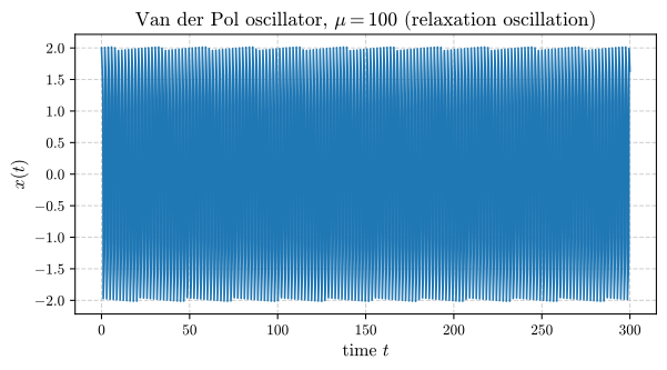
Figure 1: $x(t)$ for $\mu = 100$. The long, slow plateaus are interrupted by sudden, sharp transitions; this contrast between fast and slow timescales is the defining signature of a stiff system.
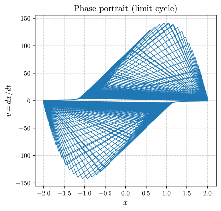
Figure 2: The corresponding phase portrait. The trajectory rapidly converges onto a limit cycle with sharp corners, which are the regions where the fast dynamics dominate.
Why stiffness constrains explicit solvers: a stability argument
The clearest route to understanding why explicit methods struggle is Dahlquist’s test equation (Dahlquist, 1963):
\[y' = \lambda y, \qquad \lambda \in \mathbb{C}, \ \mathrm{Re}(\lambda) < 0 .\]This is a linearization of the local behavior near a fast-decaying mode, precisely the kind of term that dominates the local Jacobian of a stiff system. Applying explicit (forward) Euler with step size $h$,
\[y_{k+1} = y_k + h\lambda y_k = (1 + h\lambda)\, y_k = (1 + z)\, y_k, \qquad z := h\lambda,\]| the numerical solution stays bounded only if $ | 1 + z | \le 1$. This defines the method’s region of absolute stability, the bounded disk of radius $1$ centered at $z = -1$ in the complex plane. For real negative $\lambda$, this requires |
| The constraint depends **only on $ | \lambda | $*, the fastest decay rate present in the system. It does not depend on the required accuracy of the solution, nor on how long the fast mode remains dynamically relevant after it has decayed. If the system contains *any eigenvalue with large $ | \lambda | $, corresponding to a fast, heavily damped mode, forward Euler is restricted to small steps for the entire simulation, including the long, slow intervals in which the solution varies little. |
Implicit (backward) Euler, by contrast, solves
\[y_{k+1} = y_k + h\lambda y_{k+1} \quad\Longrightarrow\quad y_{k+1} = \frac{y_k}{1 - z}, \qquad z = h\lambda .\]| For $\mathrm{Re}(\lambda) < 0$ and any $h > 0$, $ | 1 - z | > 1$ holds without exception, which implies $ | y_{k+1} | < | y_k | $ for every step size. Backward Euler is A-stable: unconditionally stable for this test equation, regardless of the magnitude of $h$. The step size can therefore be chosen on accuracy grounds alone. This is the principal reason implicit methods exist despite their higher per-step cost, and it is that cost which the Sherman-Morrison acceleration of the previous post is designed to offset when the system matrix has exploitable low-rank structure. |
Comparing stability regions directly
The two regions are easiest to compare side by side in the complex plane $z = h\lambda$.
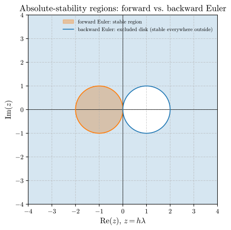
| *Figure 3: Forward Euler’s stable region is the shaded disk $ | 1+z | \le 1$ (orange); backward Euler is stable everywhere outside the disk $ | 1-z | \le 1$ (blue), which includes the entire left half-plane.* |
-
Forward Euler: the disk $ 1+z \le 1$, radius $1$, centered at $z=-1$. Any eigenvalue for which $z = h\lambda$ falls outside this disk renders the method unstable, which is why a large $ \lambda $ forces a small $h$. -
Backward Euler: the exterior of the disk $ 1-z \le 1$, which includes the entire left half-plane $\mathrm{Re}(z) \le 0$. This is the concrete meaning of “A-stable”: every eigenvalue with a negative real part is stable, for any step size. - Trapezoidal rule (Crank-Nicolson): also A-stable, and second-order accurate where backward Euler is first order. It is often the preferred default when both unconditional stability and higher accuracy are required, although it can exhibit mild oscillatory artifacts on very stiff problems that the stronger damping of backward Euler avoids.
- BDF methods (the
BDFoption inscipy.integrate.solve_ivp): a family of higher-order implicit multistep methods, A-stable up to order $2$ and only stiffly stable, a slightly weaker but still practically useful property, at higher orders (Hairer & Wanner, 1996). - Radau IIA (the
Radauoption insolve_ivp): not a multistep method but a fully implicit Runge-Kutta method. The three-stage variant used by SciPy is of order $5$ and L-stable, so it is A-stable and also strongly damps the fastest modes (Hairer & Wanner, 1996).
Production stiff solvers therefore default to BDF or Radau in preference to plain backward Euler: these methods retain the stability benefits while recovering higher-order accuracy.
Demonstrating the cost gap numerically
The Van der Pol system was solved over a short, fixed time horizon with scipy.integrate.solve_ivp (Virtanen et al., 2020), comparing an explicit method (RK45) against an implicit, stiff-aware method (Radau) across a range of $\mu$ values, and recording the number of right-hand-side evaluations and output steps each solver required to meet the same tolerance:
import numpy as np
from scipy.integrate import solve_ivp

def vdp(t, y, mu):
    x, v = y
    return [v, mu * ((1 - x**2) * v - x)]

y0 = [2.0, 0.0]
mus = [1, 10, 50, 100, 300, 600, 1000, 2000]

for mu in mus:
    sol_e = solve_ivp(vdp, (0, 4.0), y0, args=(mu,),
                      method="RK45", rtol=1e-6, atol=1e-9)
    sol_i = solve_ivp(vdp, (0, 4.0), y0, args=(mu,),
                      method="Radau", rtol=1e-6, atol=1e-9)
    print(f"mu={mu:5d}  RK45 nfev={sol_e.nfev:>8} steps={len(sol_e.t):>6}  "
          f"Radau nfev={sol_i.nfev:>6} steps={len(sol_i.t):>5}")
Results (reformatted as a table; “steps” is the number of time points returned, len(sol.t)):
mu     RK45 nfev   RK45 steps   Radau nfev   Radau steps
   1        302          41          793          105
  10       1196         171         2895          380
  50       2942         445         5230          669
 100       4508         694         6916          876
 300       8138        1285         8102         1009
 600      12524        2013         8779         1080
1000      18602        2857         9206         1132
2000      34100        5041         9874         1200
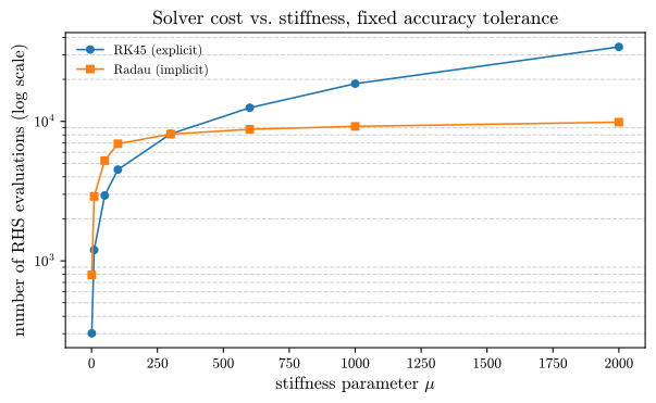
Figure 4: Number of right-hand-side evaluations required by each solver, as a function of the stiffness parameter $\mu$, on a log scale.
The horizon $t \in [0, 4]$ is much shorter than the relaxation period of the oscillator at large $\mu$ (roughly $1.6\mu$), so for the stiffer cases the benchmark measures the slow-branch regime, before the first fast transition, and not a full cycle.
The crossover occurs where the stability analysis predicts. At low stiffness, the higher per-step overhead of the implicit solver, which must solve a nonlinear system by Newton iteration at each step and therefore requires Jacobian evaluations, makes it more expensive than the explicit method. Beyond approximately $\mu \approx 300$ for this particular problem and tolerance, the cost of the explicit method continues to rise, since its step count is constrained by stability, whereas the cost growth of the implicit method flattens sharply. At $\mu = 2000$, explicit RK45 requires nearly 3.5 times as many function evaluations as the stiff-aware implicit solver.
What stiffness measures
Stiffness is not a property of an equation in isolation; it is a property of the combination of the equation, the solver, and the accuracy tolerance demanded. A system is informally called stiff when the stability-driven step-size restriction is considerably tighter than the accuracy-driven restriction would otherwise require (Curtiss & Hirschfelder, 1952). The crossover point in Figure 4 is therefore not a universal constant; it depends on the requested tolerance and the specific solver pair being compared.
Diagnosing stiffness in advance
In practice, the clean, isolated eigenvalue structure of Dahlquist’s test equation is rarely visible directly. A practical diagnostic is the stiffness ratio: compute, or estimate, the eigenvalues of the system’s local Jacobian $\partial f/\partial y$, and compare the largest and smallest rates of decay,
\[S = \frac{\max_i |\mathrm{Re}(\lambda_i)|}{\min_i |\mathrm{Re}(\lambda_i)|}.\]| The ratio is undefined when $\min_i | \mathrm{Re}(\lambda_i) | = 0$, for example at points where a Jacobian eigenvalue is purely imaginary, so it is best read as a local indicator. A large stiffness ratio ($S \gg 1$) indicates that fast and slow dynamics coexist, and that an explicit method will remain stability-constrained by the fast mode long after that mode has physically decayed to negligible magnitude. In the Van der Pol system, near the slow branch the fast eigenvalue scales roughly like $\mu$ and the slow one roughly like $1/\mu$, so $S$ grows approximately like $\mu^2$; this accounts for the predictable shift of the crossover in Figure 4 as $\mu$ increases. In production settings, most adaptive solver libraries expose the same information implicitly (Shampine & Reichelt, 1997): if the automatic step-size controller of an explicit solver repeatedly reduces the step far below what accuracy alone would demand, that behavior is a strong practical indication of a stiff system, and a reason to change solver families instead of treating the symptom. |
Summary
- Stiffness is a stability problem, not an accuracy problem: a stiff system forces small steps on an explicit solver even in regions where the solution varies little.
- The Dahlquist test equation shows why: the stability region of explicit Euler is a bounded disk, whereas that of implicit Euler covers the entire left half-plane (A-stability).
- The advantage of implicit methods is not unconditional. With mild stiffness, their per-step Newton-iteration overhead can make them more expensive than an explicit method, and the appropriate solver choice depends on where a given problem falls on that spectrum.
- This is precisely the setting in which the Sherman-Morrison acceleration of the previous post is valuable: once an implicit solver is required because a system is stiff, exploiting any low-rank structure in the evolution of the system matrix produces a performance gain at negligible additional cost.
The next post in this series addresses surrogate modeling and polynomial chaos expansion, for cases in which even a fast solver remains too expensive to evaluate thousands of times within an uncertainty-propagation loop.
References
The stability-analysis framework used throughout this post is built on Dahlquist’s original test equation and the A-stability concept (Dahlquist, 1963), as well as the classical treatment of stiffness by (Curtiss & Hirschfelder, 1952). The Van der Pol oscillator used as the running example originates with (Van der Pol, 1926). (Hairer & Wanner, 1996) is the standard reference for BDF, Radau, and other stiff-solver families, including detailed stability-region analysis; (Shampine & Reichelt, 1997) discusses practical stiffness detection and solver-switching heuristics used in production ODE software, and (Virtanen et al., 2020) documents the solve_ivp interface and solver implementations used in the benchmark above.
- Van der Pol, B. (1926). On Relaxation-Oscillations. The London, Edinburgh, and Dublin Philosophical Magazine and Journal of Science, 2(11), 978–992.
- Dahlquist, G. (1963). A Special Stability Problem for Linear Multistep Methods. BIT Numerical Mathematics, 3, 27–43.
- Hairer, E., & Wanner, G. (1996). Solving Ordinary Differential Equations II: Stiff and Differential-Algebraic Problems (2nd ed.). Springer.
- Virtanen, P., Gommers, R., Oliphant, T. E., Haberland, M., Reddy, T., Cournapeau, D., Burovski, E., Peterson, P., Weckesser, W., Bright, J., & others. (2020). SciPy 1.0: Fundamental Algorithms for Scientific Computing in Python. Nature Methods, 17, 261–272.
- Curtiss, C. F., & Hirschfelder, J. O. (1952). Integration of Stiff Equations. Proceedings of the National Academy of Sciences, 38(3), 235–243.
- Shampine, L. F., & Reichelt, M. W. (1997). The MATLAB ODE Suite. SIAM Journal on Scientific Computing, 18(1), 1–22.
Full code for this post is available in stiff_ode_demo_p2.py.