Motivation
Every earlier post in this series treated solving an equation and running the code as the same task. At the scale of a national laboratory they are not. A high-fidelity three-dimensional simulation of inertial confinement fusion, climate dynamics, or tsunami propagation can involve trillions of degrees of freedom, far more than one processor can hold in memory, let alone advance in useful time. Problems of that size can be solved only by distributing the work across thousands to millions of processors. Parallel computing is therefore not an optimization added at the end; for this class of problems it is part of the method.
Lawrence Livermore National Laboratory’s El Capitan illustrates the scale. Deployed in 2024, its theoretical peak (Rpeak) exceeds 2.79 exaflops (Lawrence Livermore National Laboratory, 2024), and in November 2024 it was verified as the fastest supercomputer in the world on the TOP500 list, which ranks systems by their measured High-Performance Linpack performance (Rmax) and not by peak, with more than 11,000 nodes joined by a high-speed interconnect (HPCwire, 2024). None of that capacity is usable without algorithms designed to be split across that many independent processors. This post builds the central such algorithm, domain decomposition, from first principles on a problem small enough for a laptop, then runs it under MPI on my own machine to see what actually limits it.
The core idea: domain decomposition
The dominant strategy for parallelizing a PDE solve is domain decomposition. The physical domain (a grid or mesh) is split into pieces, each piece is assigned to a processor, and neighboring processors exchange a thin strip of boundary data, called ghost cells or a halo, at every time step. Each processor then holds exactly enough information about its neighbors to update its own piece correctly.
A concrete problem: wave propagation from a localized source
The test problem is the two-dimensional linear wave equation (LeVeque, 2002),
\[\frac{\partial^2 u}{\partial t^2} = c^2 \left( \frac{\partial^2 u}{\partial x^2} + \frac{\partial^2 u}{\partial y^2} \right),\]with a Gaussian “uplift” pulse as the initial condition and zero initial velocity. The pulse is a simplified stand-in for the seafloor displacement that drives a tsunami. The choice is not arbitrary: a wave equation on a large spatial domain is also the model behind the LLNL-led tsunami early-warning framework that won the 2025 ACM Gordon Bell Prize (Lawrence Livermore National Laboratory, 2025), to which I return at the end.
A second-order central-difference (leapfrog) discretization in space and time gives the explicit update
\[u^{n+1}_{i,j} = 2u^n_{i,j} - u^{n-1}_{i,j} + \left(\frac{c\,\Delta t}{\Delta x}\right)^2 \left(u^n_{i+1,j} + u^n_{i-1,j} + u^n_{i,j+1} + u^n_{i,j-1} - 4u^n_{i,j}\right).\]Everything in this post rests on one structural fact: computing $u^{n+1}_{i,j}$ requires only the four nearest neighbors of $(i,j)$ at the previous step. The discrete Laplacian has support radius one in each index, so the dependency graph of the update is local, and cutting the grid into contiguous blocks creates dependencies only across block boundaries. A processor therefore needs data from its immediate neighbors, not from the whole domain, to advance its block by one step.
Splitting the grid
Let the first array index $i$ (the $x$ direction) label the rows of the grid, and suppose the $N_x$ rows are divided into $P$ contiguous blocks, one per processor. This is a one-dimensional decomposition; production codes usually decompose in two or three dimensions, for reasons discussed below. Each processor’s local array is padded with one ghost row on each side.
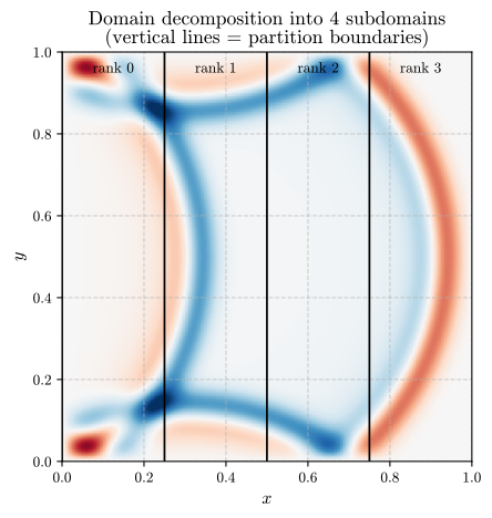
Figure 1: The wave field from the monolithic solve below, plotted with $x$ on the horizontal axis. The vertical lines mark a partition of the rows ($x$ index) into four subdomains (“ranks”), so each rank’s contiguous block of rows appears as a vertical strip spanning the full $y$ range.
At every time step, before any local computation, each rank copies its neighbors’ boundary rows into its own ghost rows. In the serial simulation of this pattern, the exchange is a pair of array copies:
# Halo exchange: each rank's ghost rows receive its neighbors' boundary rows,
# the same data movement as an MPI send-receive between neighboring ranks.
for p in range(n_procs):
    if p > 0:
        blocks_curr[p][0, :] = blocks_curr[p - 1][-2, :]    # from the left neighbor
    if p < n_procs - 1:
        blocks_curr[p][-1, :] = blocks_curr[p + 1][1, :]    # from the right neighbor
Once the ghost rows are valid, every rank computes its update independently, with no further communication until the next step:
lap_x = np.zeros_like(local_curr)
lap_x[1:-1, :] = local_curr[2:, :] + local_curr[:-2, :] - 2 * local_curr[1:-1, :]
lap_y = np.roll(local_curr, 1, axis=1) + np.roll(local_curr, -1, axis=1) - 2 * local_curr
local_next = 2 * local_curr - local_prev + r2 * (lap_x + lap_y)
This alternation, exchange boundary data and then compute locally, is the central pattern of distributed scientific computing. Nearly every parallel PDE solver follows the same two-phase structure at every step, whatever the equation.
Correctness first
Before measuring speed, I check that splitting the computation does not change the answer, the same discipline applied to the sequential solver in the first post of this series. The serial simulation of the decomposed solve is compared with a single monolithic solve on the full $240 \times 240$ grid after 300 steps:
u_mono, sensor_traces = solve_monolithic()

for n_procs in [1, 2, 4, 8, 16]:
    u_decomp = solve_decomposed(n_procs)
    max_err = np.max(np.abs(u_decomp - u_mono))
    print(f"P={n_procs:3d} subdomains: max abs difference = {max_err:.3e}")
Correctness check: decomposed solve vs monolithic solve
  P=  1 subdomains: max abs difference = 5.135e-16
  P=  2 subdomains: max abs difference = 5.135e-16
  P=  4 subdomains: max abs difference = 5.135e-16
  P=  8 subdomains: max abs difference = 5.135e-16
  P= 16 subdomains: max abs difference = 5.135e-16
The two solutions agree to round-off for every number of subdomains, as they should: with a correct halo exchange, domain decomposition is an exact reformulation of the same computation, not an approximation. The residual $5 \times 10^{-16}$ does not come from the decomposition at all. The decomposed code sums the stencil as lap_x + lap_y while the monolithic code adds the four neighbors in a different order, and floating-point addition is not associative. The MPI implementation below evaluates the stencil in exactly the monolithic order, and its result matches the monolithic solution bit for bit. When a decomposed solve disagrees with the monolithic one by more than round-off, the defect is almost always in the halo exchange; a missing or off-by-one ghost-row update is the most common bug in MPI-based PDE codes.
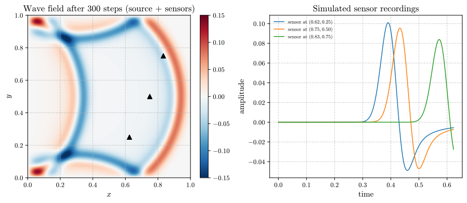
Figure 2: Left, the wave field after 300 steps, spreading outward from the Gaussian source, with black triangles marking sensor locations. Right, the amplitude recorded at each sensor over time. Inferring the source from such recordings is an inverse problem, the subject of the next post in this series.
Amdahl’s Law: the ceiling on strong scaling
With correctness established, the next question is how much faster the decomposed solve can run. The classical starting point is a result from 1967 (Amdahl, 1967). Suppose a fraction $f$ of a program’s work parallelizes perfectly across $P$ processors and the remaining fraction $1-f$ is inherently sequential (input and output, setup, or an unsplittable part of the algorithm). Amdahl’s Law gives the speedup
\[S(P) = \frac{1}{(1-f) + \dfrac{f}{P}}, \qquad \lim_{P \to \infty} S(P) = \frac{1}{1-f}.\]The speedup does not grow without bound; it approaches a hard ceiling set by the sequential fraction.
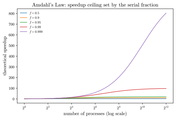
Figure 3: Theoretical speedup against the number of processes for several parallel fractions $f$. Even with 99% of the work parallelized, the speedup can never exceed $100\times$. This is a property of the arithmetic, not of any hardware.
The practical lesson is to profile before parallelizing. If a code spends 20% of its time in an unavoidably sequential phase, no amount of hardware will deliver more than a $5\times$ speedup, and requesting a larger allocation to fix a bottleneck that Amdahl’s Law has already capped wastes both compute budget and engineering time.
Weak scaling
Amdahl’s Law describes strong scaling: the problem size is fixed and processors are added. Production codes are often run in the opposite regime, weak scaling (Gustafson, 1988), where the problem grows with the processor count so that each processor keeps a fixed amount of local work. The question then is not how much faster the same problem runs, but whether $P$ times more processors can solve a $P$ times larger problem in the same wall-clock time. Gustafson’s scaled speedup expresses this regime: with $f$ now the parallel fraction of the run on $P$ processors, $S(P) = (1-f) + fP$, which grows linearly in $P$ instead of saturating (Gustafson, 1988).
The textbook obstacle to ideal weak scaling (efficiency that stays at one as $P$ grows) is communication overhead. More processors mean more halo exchanges across the interconnect, and at large enough $P$ that cost competes with the local computation.
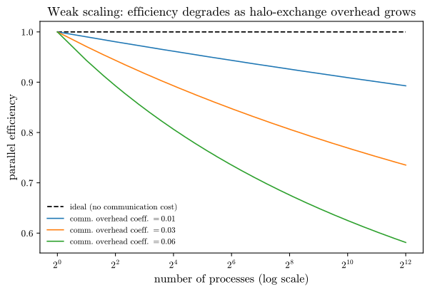
Figure 4: A simple model of weak-scaling efficiency in which communication overhead grows logarithmically with the number of processes, a crude stand-in for network topology effects. The dashed line is the ideal. Real machines add effects this model omits; the measurements below show one of them.
Communication cost is also why production codes decompose in two or three dimensions. Communication scales with the boundary each processor shares with its neighbors, while useful work scales with its interior. A one-dimensional strip has a halo that runs the full width of the domain regardless of $P$, whereas a $\sqrt{P} \times \sqrt{P}$ decomposition of an $N \times N$ grid gives each processor a square block of side $N/\sqrt{P}$, whose halo shrinks as $P$ grows. The argument is isoperimetric: compact subdomains minimize boundary relative to area, and hence communication relative to computation.
A real MPI implementation
The serial simulation above represents ranks as Python lists inside one process, which is useful for understanding and verifying the algorithm but is not parallel. A distributed implementation binds each rank to a separate process with mpi4py (Dalcı́n Lisandro et al., 2008), and the processes communicate through the Message Passing Interface (MPI) standard (Gropp et al., 2014). The core of the solver I ran, wave_mpi_p7.py, is the following loop:
# Run with, for example:  mpirun -n 8 python3 wave_mpi_p7.py --check
up = rank - 1 if rank > 0 else MPI.PROC_NULL
down = rank + 1 if rank < size - 1 else MPI.PROC_NULL

for _ in range(steps):
    # Halo exchange: send owned boundary rows, receive into ghost rows.
    comm.Sendrecv(u_curr[1], dest=up, recvbuf=u_curr[-1], source=down)
    comm.Sendrecv(u_curr[-2], dest=down, recvbuf=u_curr[0], source=up)

    # Local update, in the same arithmetic order as the monolithic solver.
    c = u_curr[1:-1]
    lap = (u_curr[:-2] + u_curr[2:]
           + np.roll(c, 1, axis=1) + np.roll(c, -1, axis=1)
           - 4 * c)
    u_next = 2 * c - u_prev[1:-1] + r2 * lap
    u_next[:, 0] = u_next[:, -1] = 0.0            # Dirichlet edges in y
    if lo == 0:
        u_next[0] = 0.0                           # top edge of the domain
    if hi == nx:
        u_next[-1] = 0.0                          # bottom edge of the domain
    u_prev[1:-1] = c
    u_curr[1:-1] = u_next
Each piece maps onto the serial simulation. Sendrecv performs the halo exchange, pairing each send with the matching receive so that neighboring ranks cannot deadlock. MPI.PROC_NULL handles the physical edges of the domain: a rank with no neighbor on one side exchanges with a null process, and the call does nothing. At the end, Gatherv reassembles the distributed rows on rank 0, where the --check option compares them with the monolithic solver.
Running it on real hardware
I ran the solver on my laptop, an AMD Ryzen 7 6800H with 8 cores and 16 hardware threads and 7.4 GiB of memory available to WSL2 Ubuntu 26.04, using Python 3.12, NumPy 2.5.3, mpi4py 4.1.2 and Open MPI 5.0.11. Ranks were pinned to physical cores up to 8 and to hardware threads beyond that, and each timing is the fastest of three runs. The driver script, bench_mpi_p7.py, and the raw results, bench_p7.json, are linked so the numbers can be reproduced.
Correctness under real MPI. For 1, 2, 4, 8, 12 and 16 ranks, the gathered field after 300 steps on the $240 \times 240$ grid differs from the monolithic solution by exactly $0$. Because the stencil is evaluated in the same order, the parallel code is not merely close to the serial one; it performs the same floating-point operations.
Strong scaling. On a $2048 \times 2048$ grid for 200 steps, the results fall well short of the ideal:
| Ranks $P$ | Wall time (s) | Speedup | Halo exchange (s) |
|---|---|---|---|
| 1 | 15.55 | 1.00 | 0.00 |
| 2 | 8.61 | 1.81 | 0.18 |
| 4 | 7.77 | 2.00 | 0.60 |
| 8 | 7.18 | 2.16 | 0.76 |
| 12 | 7.47 | 2.08 | 2.37 |
| 16 | 6.97 | 2.23 | 3.02 |
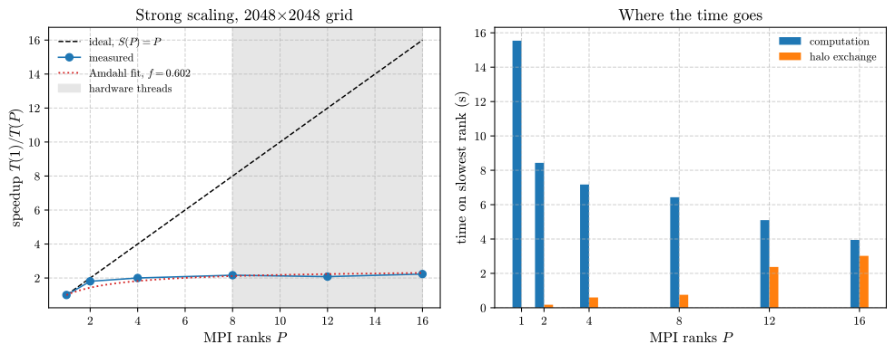
Figure 5: Left, measured speedup on a $2048 \times 2048$ grid against the ideal $S(P) = P$ and a least-squares Amdahl fit. The shaded region uses hardware threads. Right, time spent in computation and in halo exchange on the slowest rank.
Two ranks nearly halve the run time, and after that the curve is almost flat. The right panel rules out communication as the main cause up to 8 ranks: the halo exchange never exceeds 0.8 s. What stops improving is the computation itself, which falls from 15.5 s on one rank to 8.5 s on two and then only to 6.6 s on eight, even though each rank’s share of the grid keeps shrinking.
An Amdahl fit to these points returns $f \approx 0.60$, as if 40% of the program were sequential. It is not: every rank does the same fraction of the same stencil, and nothing runs serially. The fit matches the shape of the curve but describes the wrong mechanism, a useful reminder that a model which fits the data is not thereby an explanation of it.
Weak scaling makes the cause visible. With 256 rows per rank and 2048 columns, every rank does identical work at every $P$, so in the ideal case the wall time would not change. Instead the efficiency drops to 0.64 at two ranks, 0.42 at four and 0.22 at eight. The halo exchange again accounts for little of this (0.8 s at eight ranks). The computation time per rank, on the other hand, rises from 1.6 s alone to 3.7 s with four ranks and 6.6 s with eight, for exactly the same arithmetic.
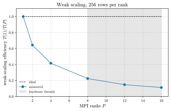
Figure 6: Measured weak-scaling efficiency with 256 rows per rank. The ideal is flat at one; the measured efficiency falls to about 0.2 at eight ranks, mostly because each rank’s local computation slows down, not because of communication.
The bottleneck is memory bandwidth
Identical work becoming slower as more cores join points to a shared resource, and on a single-socket laptop the obvious candidate is memory bandwidth. I tested this directly with a STREAM-style triad, bandwidth_p7.py, in which every rank streams through its own large arrays with no communication at all:
| Ranks $P$ | 1 | 2 | 4 | 8 | 16 |
|---|---|---|---|---|---|
| Aggregate bandwidth (GB/s) | 19.7 | 25.4 | 26.9 | 26.4 | 27.7 |
A single core already draws about 20 GB/s, and the whole chip saturates near 27 GB/s with only two ranks. Beyond that point, additional ranks divide a fixed bandwidth among themselves.
The wave-equation update is exactly the kind of kernel this penalizes. It performs about ten floating-point operations per grid point, but in NumPy every operation (each np.roll, each addition, each scalar multiplication) makes a full pass over an array in memory, so one time step moves many times more bytes than it performs floating-point operations. Such a kernel is memory-bound: its speed is set by how fast data reaches the cores, not by how fast they compute. Once two cores saturate the memory channels, the remaining six add almost nothing, which is why the strong-scaling speedup stalls near $2\times$.
This result does not contradict the case for domain decomposition; it sharpens it. On a cluster, each node brings its own memory channels, so distributing a memory-bound stencil across nodes multiplies the available bandwidth along with the compute. Within a node, the remedies are to raise the kernel’s arithmetic intensity: fuse the separate NumPy passes into a single loop (with Numba, Cython or C), tile the grid so that data are reused while still in cache, or move the kernel to a GPU, whose high-bandwidth memory can be roughly two orders of magnitude faster than a laptop’s. The same laptop that shows a $2\times$ ceiling here would show a very different curve for a compute-bound kernel.
The runs beyond eight ranks add a second, smaller effect. Ranks 9 to 16 share physical cores with ranks 1 to 8 through simultaneous multithreading, and the halo-exchange time grows from 0.8 s at eight ranks to 3.0 s at sixteen. On a machine with more cores than memory bandwidth, the scaling curve is set by memory long before communication or Amdahl’s sequential fraction come into play.
A second axis of parallelism: inside each node
Everything above concerns parallelism across processes that communicate by message passing. Modern supercomputers add a second, orthogonal axis inside each node. Each El Capitan node is built around AMD Instinct MI300A APUs, which combine CPU cores, GPU cores and a shared pool of high-bandwidth memory in one package. Using such a machine well requires two programming models at once:
- MPI (distributed-memory parallelism): the domain decomposition treated throughout this post, splitting the problem across processes that hold private memory and communicate explicitly.
-
GPU data parallelism (shared memory, SIMD-style): within a node, a GPU applies the same arithmetic to thousands of data elements simultaneously. The local update above has exactly that structure; for example,
lap_x[1:-1, :] = local_curr[2:, :] + local_curr[:-2, :] - 2 * local_curr[1:-1, :]computes every grid point’s contribution with an identical expression, independent of every other point. That independence is what thousands of lightweight GPU cores exploit, and the high-bandwidth memory beside them addresses precisely the bottleneck measured on my laptop.
Combining MPI between nodes with GPU parallelism within them is called a hybrid programming model, and it is close to universal on exascale machines. Production codes express both layers explicitly: MPI calls like those above for inter-node communication, and a GPU interface such as CUDA or HIP, or a portability layer such as Kokkos or RAJA (both developed in part at LLNL), for the node-local computation.
Exascale tsunami forecasting
The Gordon Bell Prize-winning tsunami system mentioned earlier shows these ideas at their practical limit. It used El Capitan to run the largest unstructured-mesh finite-element simulation to date, resolving 55.5 trillion degrees of freedom (Lawrence Livermore National Laboratory, 2025). That scale is out of reach for any single processor or modest cluster; it requires the decomposition-plus-halo-exchange pattern described here, spread across more than 46,000 accelerator processing units and more than 11 million CPU cores (Lawrence Livermore National Laboratory, 2025).
What makes the system more than a demonstration of scale is its inverse half. Beyond running forward simulations, the team built a framework that rapidly infers the seafloor displacement most consistent with real-time pressure-sensor data (Lawrence Livermore National Laboratory, 2025), producing forecasts about ten billion times faster than conventional approaches, in a fraction of a second (Newswise, 2025). Reasoning from noisy sensor measurements back to the unknown source is the subject of the next post in this series, and the wave-source problem in Figure 2 is a reduced version of that inference task.
Summary
- Locality makes parallelism possible. The finite-difference stencil touches only nearest neighbors, which is what allows domain decomposition to split the problem without changing the answer.
- Exchange halos, then compute locally. This two-phase pattern underlies nearly all distributed PDE solvers, whatever the equation.
- Verify correctness before measuring speed. Here the MPI solver reproduces the monolithic solution exactly; a decomposed solve that disagrees by more than round-off almost always has a halo-exchange bug.
- Amdahl’s Law is a ceiling, not a diagnosis. A fitted parallel fraction can match measured speedups while describing the wrong mechanism, as the $f \approx 0.60$ fit to my laptop runs does.
- On a single node, memory bandwidth often binds first. A memory-bound stencil stopped scaling at about two ranks on my laptop because two cores already saturate the memory system; distributing across nodes, fusing operations, or moving to high-bandwidth GPU memory addresses this, while more cores on the same socket do not.
- At scale, communication and decomposition geometry matter. Two- and three-dimensional decompositions reduce halo size relative to useful work, which is why production codes prefer them.
References
The theoretical framework follows (Amdahl, 1967) for strong scaling and (Gustafson, 1988) for weak scaling. (Gropp et al., 2014) is the standard reference for MPI programming and the domain-decomposition patterns used here, and (Dalcı́n Lisandro et al., 2008) documents mpi4py. (LeVeque, 2002) covers the discretization and stability of the wave equation. The El Capitan details are drawn from (Lawrence Livermore National Laboratory, 2024) and (HPCwire, 2024), and the Gordon Bell Prize-winning tsunami system from (Lawrence Livermore National Laboratory, 2025) and (Newswise, 2025).
- Lawrence Livermore National Laboratory. (2024). El Capitan: NNSA’s First Exascale Machine. Advanced Simulation and Computing Program. https://asc.llnl.gov/exascale/el-capitan
- HPCwire. (2024). LLNL’s El Capitan Verified as World’s Fastest Supercomputer. https://www.hpcwire.com
- LeVeque, R. J. (2002). Finite Volume Methods for Hyperbolic Problems. Cambridge University Press.
- Lawrence Livermore National Laboratory. (2025). LLNL, UT & UCSD Win Gordon Bell Prize with Exascale Tsunami Forecasting. https://www.llnl.gov/article/53636
- Amdahl, G. M. (1967). Validity of the Single Processor Approach to Achieving Large Scale Computing Capabilities. AFIPS Spring Joint Computer Conference, 483–485.
- Gustafson, J. L. (1988). Reevaluating Amdahl’s Law. Communications of the ACM, 31(5), 532–533.
- Dalcı́n Lisandro, Paz, R., Storti, M., & D’Elı́a Jorge. (2008). MPI for Python: Performance Improvements and MPI-2 Extensions. Journal of Parallel and Distributed Computing, 68(5), 655–662.
- Gropp, W., Lusk, E., & Skjellum, A. (2014). Using MPI: Portable Parallel Programming with the Message-Passing Interface (3rd ed.). MIT Press.
- Newswise. (2025). LLNL, UT & UCSD Win Gordon Bell Prize with Exascale Tsunami Forecasting. https://www.newswise.com/articles/llnl-ut-ucsd-win-gordon-bell-prize-with-exascale-tsunami-forecasting
Code for this post: the serial demonstration and Figures 1 to 4, hpc_domain_decomposition_p7.py; the MPI solver, wave_mpi_p7.py; the benchmark driver and plotting script for Figures 5 and 6, bench_mpi_p7.py and plot_bench_p7.py; the bandwidth test, bandwidth_p7.py; and the raw measurements, bench_p7.json and bandwidth_p7.json.