Optimization: Gradient, Newton and Quasi-Newton Methods and Minimum-Energy Trajectory Optimization

Motivation: the problem underneath the rest of this series

Almost every earlier post in this series has contained an optimization problem in disguise: fitting a surrogate model, training a PINN, or computing a maximum-likelihood or maximum-a-posteriori estimate, as in the previous post on Bayesian inference. This post makes that structure the explicit subject. It starts from the mathematical guarantees that make some optimization problems provably easy, moves through the algorithms that exploit those guarantees, and ends with a non-convex problem (optimal trajectory design) where those guarantees no longer hold and different tools are needed.

Convexity: the property that makes optimization tractable

A function $f: \mathbb{R}^n \to \mathbb{R}$ is convex if, for any two points $x, y$ and any $\lambda \in [0,1]$,

Geometrically, the line segment connecting any two points on the graph of $f$ never lies below the graph. If $f$ is twice differentiable, an equivalent and often more easily checked condition is that its Hessian matrix is positive semi-definite everywhere (Boyd & Vandenberghe, 2004),

Why this single property matters

For a convex function, every local minimum is a global minimum, so there are no other valleys in which to become trapped. The argument follows directly from the definition. Suppose $x^\star$ is a local but not global minimum, so that some $y$ satisfies $f(y) < f(x^\star)$. Convexity forces $f$ along the segment from $x^\star$ to $y$ to lie at or below the chord connecting them, and that chord strictly decreases from $f(x^\star)$; points arbitrarily close to $x^\star$ therefore have smaller values, which contradicts local optimality. The practical consequence is substantial: an algorithm applied to a convex problem comes with a mathematical guarantee of reaching the global optimum, whereas the same algorithm applied to a non-convex problem does not. This is also why applied mathematicians put effort into recognizing convexity, or building it into a formulation, even at the cost of a less “natural” model. Regularized linear and logistic regression, support vector machines, and the LASSO are all formulated to be convex so that their optimization step is provably reliable.

The workhorse problem: logistic regression as a convex optimization problem

To make this concrete with real data, this section returns to the breast cancer diagnostic dataset used in the machine learning toolkit post, where logistic regression was the best-performing model, and treats fitting a logistic regression classifier as what it is: minimizing a convex loss function. The $L_2$-regularized negative log-likelihood is

where $\sigma(z) = 1/(1+e^{-z})$ is the sigmoid function, $n$ is the number of training samples, and $\beta \in \mathbb{R}^d$. The convexity claim can be verified directly. The Hessian of this loss is

Since $\sigma(z)(1-\sigma(z)) \geq 0$ for every $z$, $W$ has non-negative diagonal entries, which makes $X^\top W X$ positive semi-definite for any $X$: for any vector $v$, $v^\top X^\top W X v = \sum_i W_{ii}(x_i^\top v)^2 \ge 0$. Adding $\frac{\lambda}{n}I$ with $\lambda > 0$ makes the whole Hessian strictly positive definite everywhere. The regularized logistic loss is therefore strictly convex regardless of the dataset it is fit to; this is a general proof, not an empirical observation about this particular dataset.

Three optimizers, one convex problem, different convergence

The same model is fit three ways below. Because the problem is convex, the final answers should agree, and they do; the interesting comparison is how quickly each method gets there, which is where the mathematical differences appear.

Gradient descent: first-order, cheap steps

def gradient_descent(X, y, n_iter=500, lr=0.5):
    beta = np.zeros(X.shape[1])
    losses = [neg_log_likelihood(beta, X, y)]
    for _ in range(n_iter):
        beta = beta - lr * gradient(beta, X, y)
        losses.append(neg_log_likelihood(beta, X, y))
    return beta, losses

beta_gd, losses_gd = gradient_descent(X_train, y_train, n_iter=500, lr=0.9)

Gradient descent uses only local slope information. It has no notion of the curvature of the loss surface, so it can zigzag across narrow, curved valleys, and its convergence rate depends on the step size $\eta$ and on the condition number $\kappa = \lambda_{\max}(\nabla^2\mathcal{L})/\lambda_{\min}(\nabla^2\mathcal{L})$, the ratio of the largest to the smallest Hessian eigenvalue. For a strongly convex quadratic with $\eta \in (0, 2/\lambda_{\max})$ the iteration converges, and with the optimal fixed step $\eta = 2/(\lambda_{\max}+\lambda_{\min})$ the error contracts by a factor of $\frac{\kappa-1}{\kappa+1}$ per step (Nocedal & Wright, 2006). This is linear convergence, and the factor approaches $1$ (arbitrarily slow progress) as $\kappa$ grows.

Newton’s method: second-order, expensive but better-informed steps

def newtons_method(X, y, n_iter=20):
    beta = np.zeros(X.shape[1])
    losses = [neg_log_likelihood(beta, X, y)]
    for _ in range(n_iter):
        g = gradient(beta, X, y)
        H = hessian(beta, X, y)
        beta = beta - np.linalg.solve(H, g)
        losses.append(neg_log_likelihood(beta, X, y))
    return beta, losses

Newton’s method uses the full local curvature (the Hessian) to rescale the step. Geometrically, it fits a quadratic model of the loss at the current point and jumps to the minimizer of that model instead of taking a small step along the gradient. Near a minimizer with a Lipschitz-continuous, positive definite Hessian, this gives quadratic convergence: the number of correct digits roughly doubles every iteration, a much faster asymptotic rate than the linear convergence of gradient descent (Nocedal & Wright, 2006). The script uses the pure (undamped) Newton step, which converged here from $\beta = 0$; in general a line search or damping is needed to guarantee convergence from a distant starting point. The cost is also real: forming and factorizing a $d \times d$ Hessian costs $O(d^3)$ per iteration (the same cost structure discussed in the first post of this series), which is why Newton’s method is impractical for the very high-dimensional parameter spaces common in deep learning.

L-BFGS: approximating the Hessian without forming it

Between these two extremes sits L-BFGS (limited-memory Broyden-Fletcher-Goldfarb-Shanno) (Liu & Nocedal, 1989), which also trained the PINN in an earlier post in this series. L-BFGS builds an implicit approximation to the inverse Hessian from only the most recent gradient and step pairs. Each BFGS update is a rank-two correction, and the corresponding inverse update is an instance of the Sherman-Morrison-Woodbury identity from the first post of this series; here it accumulates curvature information instead of solving a fixed linear system with a changing low-rank correction. The same linear-algebra idea that accelerated an ODE solver in that post is what makes practical quasi-Newton optimization work. Full BFGS converges superlinearly near a well-behaved minimizer; the limited-memory variant is in general guaranteed only a linear rate, but in practice it is usually much faster than gradient descent (Nocedal & Wright, 2006).

res = minimize(neg_log_likelihood, beta0, args=(X, y), jac=gradient,
                method="L-BFGS-B", callback=callback,
                options=dict(maxiter=200))

Convergence results on the breast cancer dataset

Running optimizers on full 30-feature logistic regression...
Final training loss -- GD: 0.068652 (500 iters)
Final training loss -- Newton: 0.068537 (20 iters)
Final training loss -- L-BFGS: 0.068537 (28 iters)
Test accuracy -- GD: 0.9860
Test accuracy -- Newton: 0.9860
Test accuracy -- L-BFGS: 0.9860

All three methods reach the same test accuracy, and Newton’s method and L-BFGS agree on the training loss to six decimal places, as convexity leads one to expect. Newton’s method reaches the minimum to within numerical precision in fewer than 10 of its 20 iterations, whereas gradient descent, after 500 iterations, is still about $10^{-4}$ above it (0.068652 versus 0.068537).

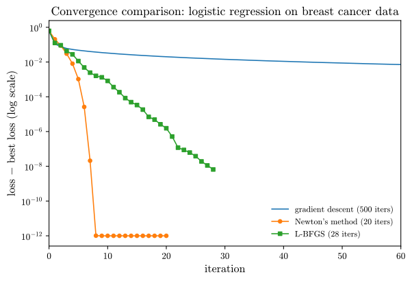
Figure 1: Gap between the loss and the best loss found, per iteration, on a log scale (first 60 iterations shown). Newton’s method (orange) falls from about $10^{-2}$ to the $10^{-12}$ plotting floor within a few iterations, the signature of quadratic convergence. L-BFGS (green) decreases steadily to about $10^{-8}$ in 28 iterations without forming the Hessian. Gradient descent (blue) is still near $10^{-2}$ after 60 iterations.

The loss landscape and optimizer paths

To visualize the difference, the model can be restricted to 2 of the 30 features (mean radius and mean texture), so that the convex loss surface can be plotted with each optimizer’s path overlaid.

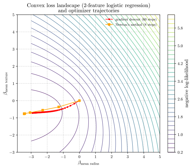
Figure 2: Contours of the 2-feature loss surface, which has a single basin, as convexity requires. Both methods start at the origin. Gradient descent (red, 60 steps) takes many short steps whose length shrinks as it moves into the flat, elongated part of the basin, and it stops short of the point reached by Newton’s method. Newton’s method (orange, 8 steps) takes a few long steps because it accounts for the curvature and anisotropy of the basin directly.

The figure shows the geometric content of the argument above: Newton’s method uses the Hessian to account for the shape of the basin at every step, while gradient descent proceeds using only the local slope and slows down where the surface flattens.

A necessary detour: what “constrained optimum” means

Before turning to trajectory optimization, it helps to state what it means, mathematically, for a point to be optimal subject to constraints. A problem simple enough to visualize completely serves this purpose.

Consider minimizing $f(x,y) = x^2 + y^2$ (squared distance from the origin) subject to $g(x,y) = x + y - 2 = 0$ (staying on a fixed line). At the constrained optimum, the level curves of $f$ (concentric circles) must be tangent to the constraint line: if a circle crossed the line instead of touching it, sliding along the line would reach a smaller circle. Tangency means the gradients are parallel,

for some scalar $\lambda$, the Lagrange multiplier. This equation, together with $g(x,y)=0$, gives exactly enough equations to solve for $(x, y, \lambda)$. Here $\nabla f = (2x, 2y)$ and $\nabla g = (1,1)$, so $2x = \lambda = 2y$ and hence $x=y$; combined with $x+y=2$, this gives $x=y=1$ and a minimum value $f(1,1)=2$. The result is easy to verify by direct substitution, which is a good habit whenever a Lagrangian calculation is new.

The Karush-Kuhn-Tucker (KKT) conditions generalize this idea to inequality constraints $h(x) \le 0$ (Karush, 1939)(Kuhn & Tucker, 1951). At a constrained optimum (under a suitable constraint qualification), each inequality constraint is either inactive, in which case it contributes nothing, or active, in which case it contributes a multiplier term to the gradient balance as in the equality case, with the added requirement that its multiplier be non-negative. The sign condition formalizes the statement that pushing against an active constraint is what prevents further improvement. The dynamics_constraints and boundary_constraints functions in the trajectory problem below are equality constraints in exactly this Lagrangian sense, and SLSQP works by solving a sequence of quadratic-programming approximations to these optimality conditions.

Beyond convexity: trajectory optimization

Convexity is valuable when available, but many physically interesting control and design problems lack it. To see what changes, consider a minimum-fuel trajectory optimization problem, a simplified one-dimensional stand-in for the kind of aviation trajectory problem referenced elsewhere in this series (and related to the LLNL sustainable-aviation modeling project from which this series grew).

The problem

A vehicle with position $q(t)$ and velocity $v(t)$ is driven by a control input $u(t)$ (thrust) against quadratic drag,

with $k = 0.02$ in the script. Starting from rest at $q(0)=0$, the goal is to reach $q(T) = q_f$ with zero final velocity at $T = 10$, with $q_f = 20$, while minimizing fuel usage. Fuel is approximated here by $\int_0^T u(t)^2\,dt$, a smooth proxy (strictly a control-energy cost) that keeps the problem gradient-friendly:

How this differs from the logistic regression problem

Direct collocation: from a function-optimization problem to a finite one

The standard practical approach, direct collocation (Betts, 2010), discretizes time into $N$ nodes (60 in the script) and treats the state and control values at each node as ordinary optimization variables. The dynamics are then enforced as equality constraints connecting consecutive nodes, here via the trapezoidal rule:

def dynamics_constraints(z):
    q, v, u = unpack_traj(z)
    cons = []
    for k in range(N_NODES - 1):
        # trapezoidal collocation for q and v
        drag_k = DRAG_COEF * v[k] * np.abs(v[k])
        drag_k1 = DRAG_COEF * v[k+1] * np.abs(v[k+1])
        q_next_pred = q[k] + 0.5 * dt_traj * (v[k] + v[k+1])
        v_next_pred = v[k] + 0.5 * dt_traj * ((u[k] - drag_k) + (u[k+1] - drag_k1))
        cons.append(q[k+1] - q_next_pred)
        cons.append(v[k+1] - v_next_pred)
    return np.array(cons)

This converts the continuous-time problem into a finite-dimensional nonlinear program with 180 variables, which is solved with Sequential Least Squares Programming (SLSQP) (Kraft, 1988), a general-purpose sequential quadratic programming method for constrained nonlinear problems. The initial guess is a straight-line position profile, a constant velocity, and zero control.

constraints = [
    {"type": "eq", "fun": dynamics_constraints},
    {"type": "eq", "fun": boundary_constraints},
]
result = minimize(objective, z0, constraints=constraints, method="SLSQP",
                   options=dict(maxiter=300, ftol=1e-9))

PART B: Minimum-fuel trajectory optimization
Optimization success: True, message: Optimization terminated successfully
Final fuel cost (integral of u^2): 4.9367

A useful check is available. Without drag ($k = 0$) the problem is the classical minimum-energy rest-to-rest transfer of a double integrator, whose optimal control is linear in time, $u^\star(t) = \frac{6 q_f}{T^2}\left(1 - \frac{2t}{T}\right)$, with minimum cost $12 q_f^2 / T^3$. For $q_f = 20$ and $T = 10$ this gives $4.8$. The computed cost of 4.9367 is about 3% higher, which is consistent with the additional thrust needed to overcome the small drag term.

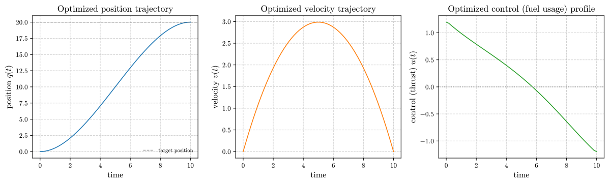
Figure 3: The optimized position, velocity, and control (thrust) trajectories. The control decreases almost linearly from about $1.2$ to about $-1.2$, changing sign shortly before $t = 6$; the velocity rises to a peak of about $3$ near $t = 5$ and returns to zero at $t = 10$, and the position reaches the target of 20 smoothly. The near-linear control is close to the drag-free analytic optimum; the drag term shifts the sign change slightly later than the midpoint, since some thrust is needed to counter drag.

What “solved” means here

Unlike the logistic regression example, result.success = True here means that SLSQP found a point satisfying the KKT conditions to within tolerance. These are first-order necessary conditions for a local constrained optimum, not a certificate of global optimality. For a problem this simple (smooth, low-dimensional, with one sensible physical strategy, and close to a convex drag-free problem) the local optimum found is very likely the global one, but that is a statement about this particular problem, not a guarantee provided by SLSQP. For more complex trajectory problems (multiple obstacles, discrete mode switches, highly oscillatory dynamics), practitioners commonly run the optimizer from several initial guesses and compare the results, because a single successful run does not rule out a better solution elsewhere in the search space.

Neural networks at the intersection of optimization and physics-informed learning

An active research direction, which connects back to the PINN post earlier in this series, uses neural networks inside the optimization loop for trajectory and control problems, not only as forward PDE solvers. Instead of parameterizing the control $u(t)$ at a fixed set of collocation nodes, as above, a small neural network $u_\theta(t)$ can represent the control as a smooth function of time, with the network weights as the optimization variables. A related line of work uses deep networks to approximate solutions of the Hamilton-Jacobi-Bellman equation and hence optimal feedback controls in high dimensions (Nakamura-Zimmerer et al., 2021). These approaches are attractive for high-dimensional state spaces and for settings in which the dynamics are only partially known and must be learned from data along with the control, which is a different regime from the fully known dynamics solved by direct collocation above. The trade-offs mirror those in the PINN post: a more flexible representation and easier handling of high-dimensional state spaces, at the cost of the convergence guarantees that a well-posed classical collocation method provides when the dynamics are fully known. Understanding both approaches, and when each is appropriate, is more useful than treating either as a replacement for the other.

Summary

• Convexity is a provable, checkable property (for example, via the Hessian), and determining whether a problem is convex is one of the first steps in choosing a solution method: it separates a guaranteed global optimum from a possibly local one.
• Newton’s method converges much faster than gradient descent near a solution (quadratic versus linear convergence) by using curvature information, at the cost of an $O(d^3)$ Hessian solve per iteration, the same cost/benefit trade-off explored with the Sherman-Morrison formula in the first post of this series.
• L-BFGS obtains much of Newton’s benefit without forming the Hessian, by building an implicit low-rank approximation from recent gradient history using the same rank-update mathematics as the Sherman-Morrison acceleration technique.
• Direct collocation is the standard practical bridge from a continuous-time, infinite-dimensional control problem to a finite, numerically solvable one, turning the dynamics into equality constraints.
• A successful non-convex optimization run guarantees only a local optimum, so on problems that are not provably convex it is worth checking the result against multiple starting points or a known reference solution, as with the drag-free cost of 4.8 above.

The next post turns to computational fluid dynamics.

References

The convexity theory and algorithms in Part A follow (Boyd & Vandenberghe, 2004) and (Nocedal & Wright, 2006), with the L-BFGS method due to (Liu & Nocedal, 1989). The KKT optimality conditions trace back to (Karush, 1939) and (Kuhn & Tucker, 1951). (Wright, 2015) offers a complementary perspective on first-order methods beyond plain gradient descent. The SLSQP algorithm used for trajectory optimization in Part B is due to (Kraft, 1988), with (Betts, 2010) as a standard reference for direct collocation, and (Nakamura-Zimmerer et al., 2021) as an example of recent neural-network-based work on optimal control.

1. Boyd, S., & Vandenberghe, L. (2004). Convex Optimization. Cambridge University Press.
2. Nocedal, J., & Wright, S. J. (2006). Numerical Optimization (2nd ed.). Springer.
3. Liu, D. C., & Nocedal, J. (1989). On the Limited Memory BFGS Method for Large Scale Optimization. Mathematical Programming, 45(1), 503–528.
4. Karush, W. (1939). Minima of Functions of Several Variables with Inequality Constraints [Master's thesis]. University of Chicago.
5. Kuhn, H. W., & Tucker, A. W. (1951). Nonlinear Programming. Proceedings of the Second Berkeley Symposium on Mathematical Statistics and Probability, 481–492.
6. Betts, J. T. (2010). Practical Methods for Optimal Control and Estimation Using Nonlinear Programming (2nd ed.). SIAM.
7. Kraft, D. (1988). A Software Package for Sequential Quadratic Programming (No. DFVLR-FB 88-28; Issue DFVLR-FB 88-28). Institut für Dynamik der Flugsysteme, DFVLR.
8. Nakamura-Zimmerer, T., Gong, Q., & Kang, W. (2021). Adaptive Deep Learning for High-Dimensional Hamilton-Jacobi-Bellman Equations. SIAM Journal on Scientific Computing, 43(2), A1221–A1247.
9. Wright, S. J. (2015). Coordinate Descent Algorithms. Mathematical Programming, 151(1), 3–34.

Code: the full script for the logistic regression optimizer comparison and the trajectory optimization example is available as optimization_p9.py.