Physics-Informed Neural Networks versus Adaptive Runge-Kutta: Accuracy and Cost on a Forced Linear ODE

Motivation

The first three posts in this series worked entirely within classical numerical analysis: fast linear algebra in the Sherman-Morrison post, stability-aware time integration in the stiff-ODE post, and polynomial-based surrogate modeling in the uncertainty-quantification post. A natural next step is to examine physics-informed neural networks (PINNs) (Raissi et al., 2019), which are widely represented in the scientific machine learning literature and are frequently presented as a general-purpose replacement for classical PDE and ODE solvers.

This post examines that claim quantitatively, without either dismissing PINNs outright or accepting the prevailing enthusiasm uncritically. As with most comparisons of tools in applied mathematics, the conclusion is conditional: performance depends on the problem, and specifying what it depends on is more useful than a general verdict in either direction.

What a PINN is

A PINN approximates the solution of a differential equation with a neural network $\hat{y}(t; \theta)$, trained not on labeled solution data but on the residual of the governing equation itself. The idea of training a network to satisfy a differential equation predates the current terminology; an early formulation appears in (Lagaris et al., 1998). For an ODE $\dot{y} = g(t, y)$, the training loss is built from

evaluated at a set of collocation points $t_i$ sampled across the domain, with a penalty weight $\lambda > 0$ on the initial condition. Training minimizes this loss over the network’s parameters $\theta$, using automatic differentiation, or closed-form derivatives for sufficiently small networks, to compute $d\hat{y}/dt$ exactly as a function of $\theta$.

A PINN therefore embodies a different computational paradigm from advancing a solution forward in time. Instead of marching through the domain, a PINN solves a global nonlinear optimization problem over the entire domain at once, exchanging the guaranteed local error control of a time-stepping method for the flexibility of a mesh-free function approximator.

A test problem with a known exact solution

To ensure the comparison is well posed, I chose a problem simple enough to admit a closed-form solution, so that both methods are scored against ground truth and not merely against each other: a forced, damped linear ODE representing Newton cooling with an oscillating ambient temperature,

with $k=2$, $A=1$, $\omega=3$, $y_0 = 0.3$, solved over $t \in [0, 3]$. This is a first-order linear ODE, solvable exactly via an integrating factor: multiplying through by $e^{kt}$ turns the left-hand side into an exact derivative,

which integrates in closed form to

The sign of the homogeneous coefficient follows from the initial condition: the particular solution satisfies $y_p(0) = -kA\omega/(k^2+\omega^2)$, so the coefficient of $e^{-kt}$ must be $y_0 - y_p(0) = y_0 + kA\omega/(k^2+\omega^2)$. Because the exact solution is available, any discrepancy between a numerical method and the truth is unambiguous and cannot be an artifact of an unknown reference.

Building a minimal PINN without a deep learning framework

Because this is a first-order ODE, only a first derivative of the network output is required, which permits the network and its exact analytic time-derivative to be written in closed form for a single-hidden-layer tanh network,

and trained with a standard gradient-based optimizer, with no automatic differentiation framework required. The penalty weight $\lambda$ in the loss above is the constant 50.0 in the code:

import numpy as np
from scipy.optimize import minimize

# Problem definition (as in the full script)
k, A, omega, y0 = 2.0, 1.0, 3.0, 0.3

def rhs(t, y):
    return -k * (y - A * np.sin(omega * t))

n_hidden = 12

def unpack(theta):
    w1 = theta[0:n_hidden]
    b1 = theta[n_hidden:2*n_hidden]
    w2 = theta[2*n_hidden:3*n_hidden]
    b2 = theta[3*n_hidden]
    return w1, b1, w2, b2

def y_hat(t, theta):
    w1, b1, w2, b2 = unpack(theta)
    z = np.outer(t, w1) + b1
    return np.tanh(z) @ w2 + b2

def dy_hat_dt(t, theta):
    w1, b1, w2, b2 = unpack(theta)
    z = np.outer(t, w1) + b1
    dh = (1 - np.tanh(z)**2) * w1     # d/dt[tanh(w1 t + b1)]
    return dh @ w2

def loss(theta, t_colloc):
    y = y_hat(t_colloc, theta)
    dy = dy_hat_dt(t_colloc, theta)
    residual = dy - rhs(t_colloc, y)               # ODE residual
    ic_pred = y_hat(np.array([0.0]), theta)[0]
    return np.mean(residual**2) + 50.0 * (ic_pred - y0)**2

t_colloc = np.linspace(0, 3.0, 60)
theta0 = 0.5 * np.random.default_rng(42).standard_normal(3*n_hidden + 1)
result = minimize(loss, theta0, args=(t_colloc,), method="L-BFGS-B",
                   options=dict(maxiter=4000, ftol=1e-14, gtol=1e-12))

The classical baseline is scipy.integrate.solve_ivp with RK45, called once, at tight tolerances (rtol=1e-10, atol=1e-12).

Results

The script was run on an AMD Ryzen 7 6800H laptop under WSL2 (Ubuntu 26.04) with Python 3.12.14, NumPy 2.5.3, and SciPy 1.18.1, using single-threaded BLAS. The timings below come from a single run and should be read as indicative of order of magnitude, not as precise benchmarks.

Classical RK45: wall=62.658 ms, max err vs exact = 3.33e-10
PINN training: wall=2960.5 ms, final loss=1.425e-03, iters=338, converged=False
PINN: max err vs exact = 1.48e-02

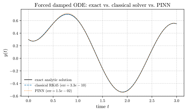
Figure 1: Exact analytic solution, classical RK45 solution, and PINN prediction. The classical solver is visually exact; the PINN captures the qualitative shape but has visible, non-trivial error.

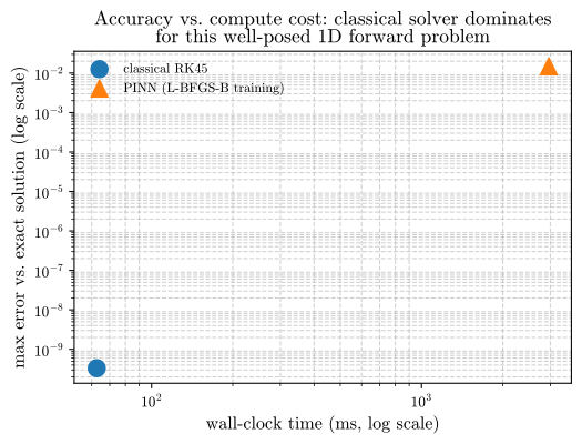
Figure 2: Accuracy against compute cost, both axes log-scaled. For this problem, the classical solver dominates on both axes simultaneously, being both faster and more accurate. No trade-off arises here; one method is strictly preferable for this specific problem class.

For this problem, the classical solver is not merely faster: its maximum error is smaller by a factor of about $4.5 \times 10^{7}$, more than seven orders of magnitude, while its wall-clock time is roughly 47 times shorter. This outcome is expected. A well-posed, smooth, low-dimensional forward ODE problem is precisely the setting for which classical numerical analysis has been refined over a century. There was no basis for expecting a general-purpose function approximator, trained from scratch by nonlinear optimization, to compete with a purpose-built, convergence-guaranteed adaptive-step solver in that regime.

When PINNs are the appropriate tool

PINNs are a reasonable tool for a different class of problem from the one above. The settings in which the trade-off shifts include:

• Inverse and parameter-inference problems. If the objective is to infer an unknown coefficient in the governing equation from sparse, noisy observations, a PINN can combine the physics residual and the data-fit term into a single loss. Classical approaches, such as a forward solver coupled to an optimizer with adjoint-based gradients, are well established and often very efficient, but they require more problem-specific machinery to set up.
• High-dimensional PDEs. Classical mesh-based methods, including finite difference and finite element schemes, suffer their own curse of dimensionality, since cost grows exponentially with spatial dimension. A mesh-free neural-network parameterization avoids discretizing a high-dimensional grid, which is valuable in high dimensions, where classical mesh generation becomes impractical (Karniadakis et al., 2021).
• Irregular geometries and mesh generation cost. For complex geometries in which generating a good-quality mesh is itself expensive or unreliable, a mesh-free method removes that requirement entirely.
• Amortized or parametric solves. If the solution is required for many different parameter settings or boundary conditions, a network trained once and conditioned on those parameters can amortize cost across queries in a manner unavailable to a classical solver re-run from scratch.

None of these characterizations describe the test problem above, and that is deliberate. The comparison is informative because I selected a problem type in which classical methods should be expected to prevail, which avoids constructing a straw comparison in either direction.

Sources of the residual PINN error

The reasons the PINN underperformed here merit explicit treatment, since they are informative about how these networks behave.

Training is a non-convex optimization problem. Unlike a classical solver, which advances with a mathematically guaranteed local error per step, the training loss of a PINN is a highly non-convex function of the network weights. L-BFGS-B stopped after 338 iterations with a final loss of approximately $1.4\times 10^{-3}$, well short of zero, and reported that its convergence criteria were not met (converged=False). A different random initialization, a different optimizer (Adam followed by a second-order refinement is a common procedure in the literature), or more training iterations may perform better, but no guarantee of convergence to the global optimum exists of the kind available for a well-posed linear solve.

Spectral bias. A well-documented phenomenon in the neural-network literature, sometimes termed the “F-principle”, is that networks trained by gradient descent tend to fit low-frequency components of a target function considerably faster than high-frequency ones (Rahaman et al., 2019)(Xu et al., 2020). For an oscillatory right-hand side such as $\sin(\omega t)$ with $\omega = 3$, this bias works directly against the PINN, and is part of the reason the residual loss plateaus instead of continuing to decrease with further iterations (Wang et al., 2022).

Collocation density and network capacity. With only 60 collocation points and 12 hidden units, the network operates within a small budget by the standards of scientific machine learning. Production PINN implementations typically use hundreds to thousands of collocation points, deeper networks, and considerably longer training runs, all of which would plausibly narrow the accuracy gap, though at a proportionally larger compute cost. For a problem of this simplicity, that additional cost reinforces the cost-accuracy conclusion above.

None of this constitutes a defense of the specific figures. Two gaps should be distinguished. The accuracy gap is largely a training artifact: it reflects non-convex optimization, spectral bias, and a small budget, and more careful training could reduce it. The cost gap is structural: any PINN must solve a global optimization problem with many residual evaluations, whereas the adaptive solver needs only a modest number of right-hand-side evaluations, so the classical solver would remain preferable on this problem under any reasonable amount of additional PINN tuning. Understanding how PINNs are trained is what permits prediction of which harder problems might shift the balance.

Summary Notes and Highlights

• Benchmarking against a known exact solution, and not only against the competing method, is what makes a comparison of this kind trustworthy.
• For smooth, low-dimensional, well-posed forward problems, classical adaptive solvers remain both faster and substantially more accurate, as should be expected.
• PINNs justify their computational cost in a different regime: inverse problems, high-dimensional PDEs, irregular geometries, and amortized multi-query settings. They are not a direct substitute for solve_ivp.
• The productive question is not whether method A is superior to method B in the abstract, but what the structure of this problem makes expensive, and which tool is designed to avoid that particular cost.

That question, namely what the structure of a specific problem makes expensive and how to avoid paying for it, has been the unifying theme of this series: exploiting low-rank structure to avoid redundant factorizations, exploiting a solver’s stability region to avoid unnecessary small steps, exploiting the smoothness of a QoI to avoid unnecessary sampling, and, in this post, assessing a method by its demonstrated strengths instead of its current prominence.

References

The PINN framework discussed throughout this post follows (Raissi et al., 2019), with earlier precedent in (Lagaris et al., 1998). (Karniadakis et al., 2021) surveys physics-informed machine learning more broadly, including the inverse-problem and high-dimensional-PDE use cases discussed above. The spectral-bias phenomenon used to explain the PINN’s training behavior is documented independently in (Rahaman et al., 2019) and (Xu et al., 2020), and (Wang et al., 2022) gives a more technical account of the training pathologies that affect PINN convergence in practice.

1. Raissi, M., Perdikaris, P., & Karniadakis, G. E. (2019). Physics-Informed Neural Networks: A Deep Learning Framework for Solving Forward and Inverse Problems Involving Nonlinear Partial Differential Equations. Journal of Computational Physics, 378, 686–707.
2. Lagaris, I. E., Likas, A., & Fotiadis, D. I. (1998). Artificial Neural Networks for Solving Ordinary and Partial Differential Equations. IEEE Transactions on Neural Networks, 9(5), 987–1000.
3. Karniadakis, G. E., Kevrekidis, I. G., Lu, L., Perdikaris, P., Wang, S., & Yang, L. (2021). Physics-Informed Machine Learning. Nature Reviews Physics, 3(6), 422–440.
4. Rahaman, N., Baratin, A., Arpit, D., Draxler, F., Lin, M., Hamprecht, F., Bengio, Y., & Courville, A. (2019). On the Spectral Bias of Neural Networks. Proceedings of the 36th International Conference on Machine Learning, 5301–5310.
5. Xu, Z.-Q. J., Zhang, Y., Luo, T., Xiao, Y., & Ma, Z. (2020). Frequency Principle: Fourier Analysis Sheds Light on Deep Neural Networks. Communications in Computational Physics, 28(5), 1746–1767.
6. Wang, S., Yu, X., & Perdikaris, P. (2022). When and Why PINNs Fail to Train: A Neural Tangent Kernel Perspective. Journal of Computational Physics, 449, 110768.

Full code for this post is available in pinn_demo_p4.py.